McKay Oil Sands 2D Seismic Inversion Case Study

Southern Pacific Resource Corp (STP) acquired 211 km of 2D seismic data in September 2007 and an additional 5.1 km2 of 3D in December 2010. The 2D survey was used as an exploration tool which ultimately led to the McKay Thermal Project. Conventional seismic interpretation has been valuable in defining the structure and regional extent of the reservoir. However, the conventional seismic character lacks the detail or consistency to delineate subtle facies variations present in the reservoir. Risk reduction through increased understanding of the reservoir at this stage of an oil sands project has the potential for significant benefits as the project moves on to production. Seismic data has already proven beneficial in the evaluation phase of this project; the intent with this case study was to investigate the potential to derive more detailed information from the seismic about the reservoir character and fluid content using quantitative interpretation (“QI”) techniques.

In order to evaluate QI seismic methods for distinguishing detailed facies types, a 15 km 2D line passing through and extending beyond the main McKay Thermal Project 3D area was selected for a feasibility project. This line (MR 2D) is regionally representative of both reservoir and non-reservoir sediments and as such the feasibility study challenged the geophysicists to answer the following questions:

• Can facies variations and fluid types be distinguished using seismic data?
• Can inversion help resolve frustrating variations in seismic response at different wells where the geology was known to be consistent?
• Can we distinguish the nature of the rocks that directly overlie the Devonian carbonates at the base of the reservoir zone?

This paper describes the results of the customized workflow designed to answer these questions and more.

Geology

The sedimentary and biogenic structures found in the main bitumen reservoir sands in the McKay Thermal Project area exhibit strong evidence of marine influence. Features such as lateral consistency and fully-marine trace fossil assemblages support the interpretation that the McKay reservoir sands belong in the Upper Marine Member of the McMurray Formation. The Upper McMurray Member is capped by the green glauconitic sands of the Wabiskaw D Member which is overlain by the Wabiskaw shale and sand (Figure 1). Both the Wabiskaw shale and sand are laterally continuous and consistent throughout the McKay project area. The Wabiskaw sand is bitumen-saturated and of interest for future prospectivity.

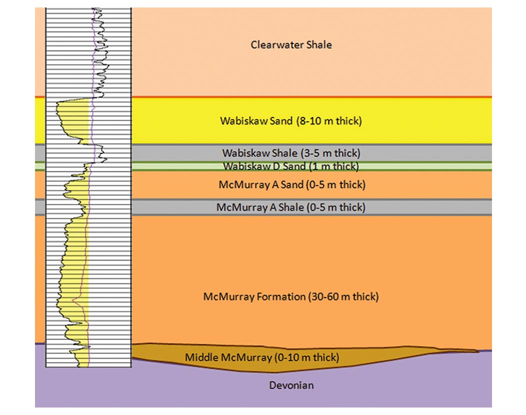
Occasional thin remnant deposits of the Middle McMurray Member are present in the lower part of the reservoir zone and consist of a mélange of discontinuous sands and muds. Although Middle McMurray sands are bitumen saturated, the zone is not considered to be part of the prospective reservoir in the project area.

Lateral changes in the reservoir sand are typically due to variability in the types and distribution of sedimentary and biogenic sedimentary structures. In cores taken from wells tying the MR 2D line, the variability in the Upper McMurray sand is largely defined by the variability in the abundance and types of biogenic sedimentary structures and the degree of preservation of the shale laminae and beds. Typically, where shale beds and laminae are present they are cross-cut by sand filled Planolites and Thalassinoides. Elsewhere the main variability is represented by the abundance and size of the Rosselia and Asterosoma. Core interpretation is essential for identifying and describing these facies, as the log response is non-specific to these distinctions. Similarly, conventional stacked seismic reflections cannot be correlated to these facies contacts; more detailed analysis is necessary.

STAC QI

To increase the resolution and accuracy of the information derived from seismic so that facies variations can be reliably predicted between wells, we use the Seismic Transformation and Classification Quantitative Interpretation (STAC QI) method. STAC QI is an integrated deterministic method that incorporates quantitative pre-stack seismic analysis calibrated to well control to predict lithology and fluid content away from the well bore. It is systematic and grounded in the reality of the rocks.

More generally, quantitative interpretation combines rock physics, empirical geological parameters, petrophysical information, and geophysical inversion techniques to predict reservoir character from seismically derived attributes. From the end-user point of view (interpreter, geologist, engineer, investor) this can lead to a bewildering maze of confusing geophysical products. We address this bewilderment with a systematic, common-sense attribute classification method based on real geology. Such an integrated method leads to more powerful results than can be observed from any single technique and contributes directly to geological understanding. Before starting the serious analysis however, we need to have confidence in our input data in order to have confidence in our output.

Data Integrity and Quality Control

Without a doubt, one of the most important steps of the quantitative interpretation process is the affirmation of quality data at the onset of the project. This is not a trivial exercise and encompasses everything from seismic processing QC to log data validation to confirmation of geological preconceptions. This case study illustrates the importance of being ruthless with data (after a fair and thorough assessment of quality) and eliminating, or at least flagging, untrustworthy data in order to achieve superior results. At the same time, we need to work with what we have. This may sound contradictory, but the entire process is nonlinear – some might say circular – and requires informed interpretive judgment throughout.

Log data can be particularly complicated. The general belief is that logs represent the truth because they come from the well. However quantitative analysis requires faith in the numbers and numbers can vary depending on normalization, calibration, depth inconsistency, processing and geology. Aside from geology, uncertainty in anything else on this list confuses the analysis, jeopardizes the validity of the outcome, and therefore must be either remedied or eliminated.

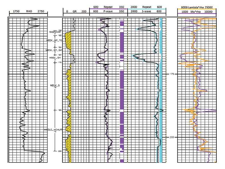
The most important logs for the quantitative interpretation process are the elastic property logs - velocity (P and S wave) and density. Borehole measurements of the P-wave (Vp) and S-wave (Vs) velocity from the dipole sonic tool are used in various stages of the seismic analysis and calibration. We assess the accuracy and consistency (hence suitability) of the log data by comparing multiple runs, other logs (from the same and other wells), core (if available) and cross-plot behavior. Figure 2 shows a QC layout for a well with poor dipole repeatability (not used in our analysis) and Figure 3 shows a well with acceptable quality.

In this project, all available wells were assessed and analyzed. After a detailed review of the data, dipole logs from two wells were judged reliable enough to use for cross-plot attribute classification and to constrain the S-wave inversion of the 2D line (although neither well tied the seismic line). Part of the quality assessment procedure is illustrated in figure 4. Cross-plots of two acoustic attributes (more about that later) for all wells are compared with those of just the two reliable wells. By eliminating poor quality data, a clear trend based on gamma-ray is visible. That doesn’t mean we ignore forevermore the wells that compliant processing flow, the basics such as NMO correction, static corrections, scaling, and migration need careful attention. Noise is almost always an issue on pre-stack data and shows up in various ways such as random, linear, multiples, side-swipe and convertedwave energy. This 2D line was reasonably clean and required only a few modifications to the conventional processing flow to preserve relative amplitudes for AVO compliance, followed by a pre-stack time migration and random noise reduction. A nearby VSP was useful in determining the correct phase (-72°) and time shift required of the seismic.

AVO

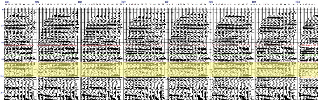
Amplitude vs Offset (AVO) analysis separates the measured pre-stack reflected amplitude into components representing P-wave, S-wave and sometimes density. The first practical step in the AVO process is to convert the prestack input data from offset domain to incident angle domain which requires an estimate of the Vp/Vs background (non-hydrocarbon) relationship and a Pwave velocity model. The velocity model is derived from P-wave sonic logs at well locations converted from depth to time and related to the interpreted seismic horizons. The Vp/Vs trend is normally determined from high quality well data, but in this case, a twowell sample was not considered sufficient to determine a locally-specific Vp/Vs trend. Based on experience, a trend was established that was guided by a regional oil-sands relationship. An example of the resulting angle gathers is shown in Figure 5. Derived incident angle is annotated at the top, ranging from 0° to 58°.

Inversion

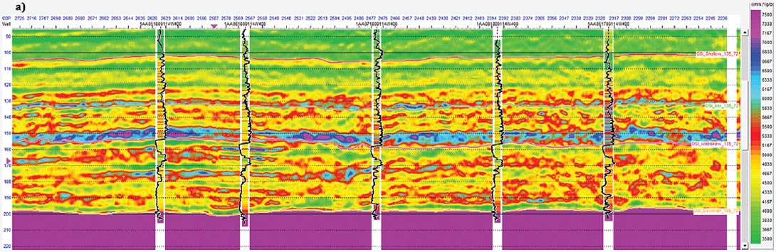
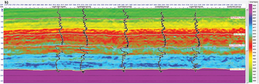
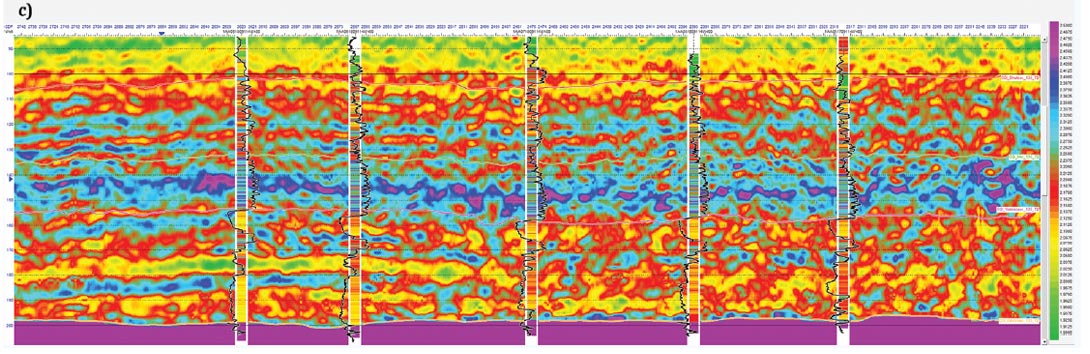
The output volumes from AVO represent P-waves, S-waves and density however they still relate only to relative impedance contrasts at layer boundaries – reflectivities. Changing reflectivities to rock layer properties requires conversion from the observed relative measurements to absolute values. The inversion method used to accomplish this for the McKay project was the model-based method (Hampson and Russell, 1990). In this approach, an initial smooth impedance model is derived from the well data and interpreted seismic horizons. The model constrains the acceptable absolute impedance range as well as supplying a low frequency trend from well logs that is lacking in seismic data. The number of wells and quality of log data incorporated at this stage has a significant effect on the accuracy and usefulness of the outcome. How many of the wells do we use in an inversion model? As Einstein said (or may have said with respect to seismic inversion): ‘Make your model as simple as possible but no simpler’. Figure 6 shows our P-impedance model for this 2D line. Figure 7 shows the inversion results for P-impedance, S-impedance and density.

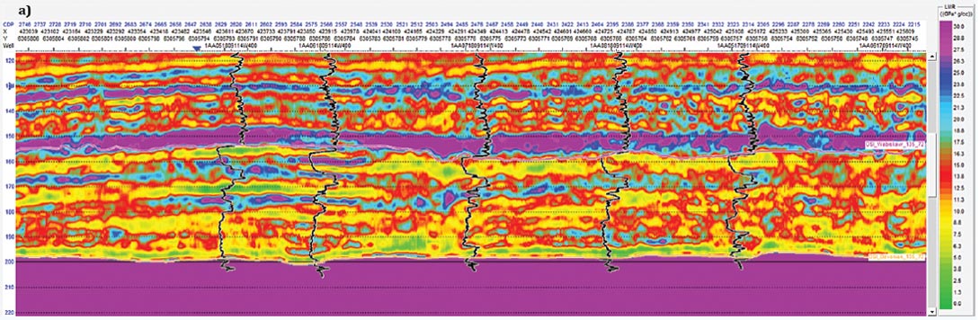
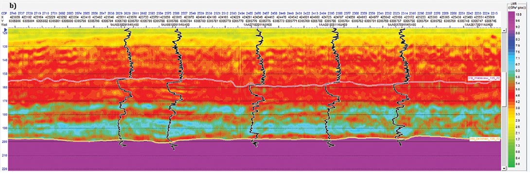
The P-impedance (Ip) and S-impedance (Is) volumes can be transformed into additional rock property volumes: Lambda*rho (incompressibility) and Mu*rho (shear rigidity) (Goodway et al., 1997) using the following equations:

μρ = Is²

λρ = Ip² – 2Is²

The results of the transformation are shown in Figure 8.

This is all very interesting so far, but what does it mean?

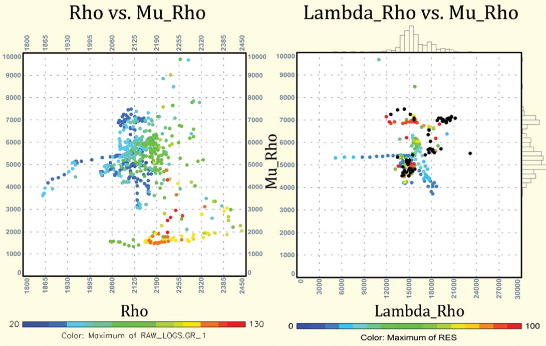
As previously alluded to, we use cross-plots of attributes to highlight distinctive relationships between these attributes that can help us quantify the elastic behavior of different rock types. By relating the calculated lambda*rho and mu*rho logs (shown in Figure 3) to the actual rock and fluid types (indicated in colour) from our two reliable wells we can establish zones and trends defined by the attributes (Figure 9).

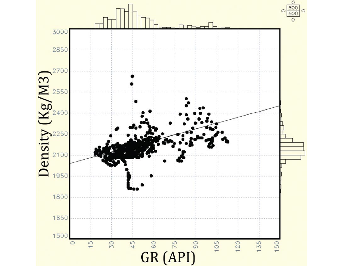
While this relationship can provide a key to unlocking the meaning of the equivalent lambda*rho and mu*rho derived from the seismic data, there is one other attribute that has an even more direct link to the rocks – density. The density vs gamma-ray plot shown in Figure 10 indicates the strong correlation between the gamma-ray indicator and the density log.

Given this link, it is definitely worth some effort to estimate density from seismic data. The density volume created by inverting an AVO estimate of density reflectivity (shown in Figure 7c) is quite noisy and uncertain (typical for this method) but appears to contain some indication of real density. We can build on that by combining it with other seismic attributes in a statistical multi-attribute analysis (Russell, et al., 1997).

Multi-attribute analysis is another form of inversion. It is a targeted process specific to a geological zone within which a particular seismic response can reasonably be expected to consistently correspond to a common geological parameter. In this analysis, the 10 wells tying the seismic data are used to statistically determine a transformation of a number of seismicallyderived attributes to reproduce a known density log at each well location. Figure 11 shows the ‘training’ data or external seismic attributes input to the process. A ranking of the attributes based on their effectiveness at reducing the error between the real log and the estimated log is created. A function incorporating the top-ranked attributes is then used to transform every trace location in the volume to a pseudo-density log (Figure 12).

Classification

To summarize the process so far: we have rigorously investigated the data for integrity and suitability. We have created attributes from seismic data as accurately as possible (calibrated by comparison with existing wells and informed judgment). And we’ve determined what those attributes mean by relating them to the rock types encountered in the wells. The next step in the process is to translate this information into spatial classification in the seismic volume.

We achieve this interactively by overlaying the seismic attribute points on the well-data cross-plots and assigning facies and fluid classes to seismic samples based on attribute cut-offs. Figure 13 shows the steps in this process. Sand and shale can be effectively separated using the density and mu*rho attributes as shown in Figure 13a which distinguishes the Clearwater shale from all other types of rock. Cross-plot (b) distinguishes the Devonian (purple) and a more detailed Wabiskaw/McMurray classification of interbedded shale (grey), mixed sand/shale facies (brown) and sand (yellow). Cross-plot (c) further distinguishes the sand into three different types which can be related to core (shown later).

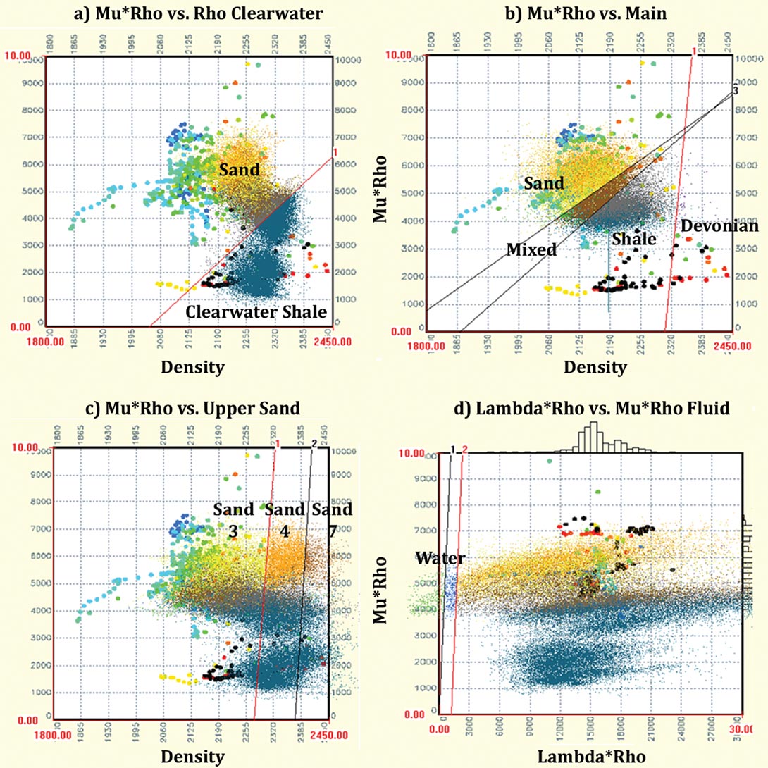
Well analysis for fluid-related attributes resulted in some encouragement that bitumen zones and low-saturation zones could be separated using the lambda*rho vs mu*rho cross-plots (shown in Figure 9). However there is insufficient representative data to have confidence in the relationship, so a regional theoretical approximation based on prior experience was applied to represent the fluid estimation. The fluid cut-offs are shown on crossplot (13d) and distinguish the depleted (or wet) zones (blue) and potential gas zones (green) from bitumen-saturated sand already classified (orange, yellow and brown).

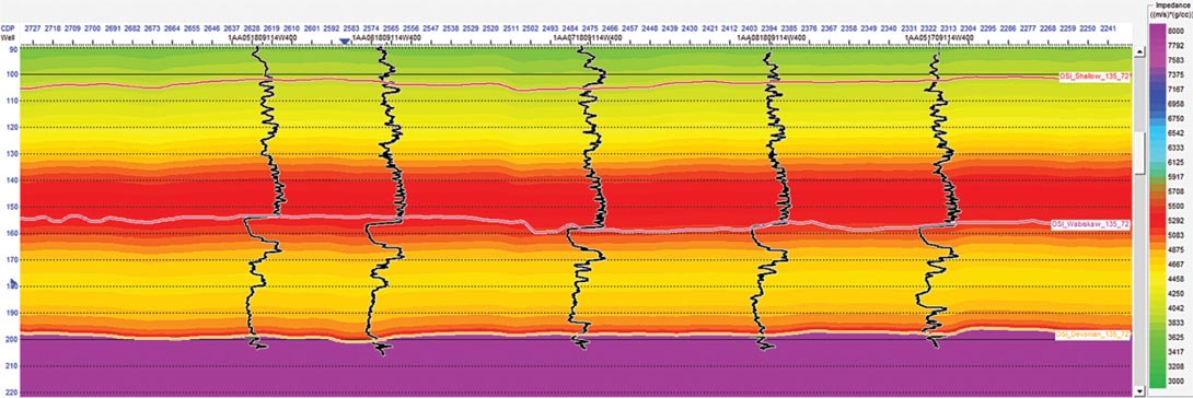
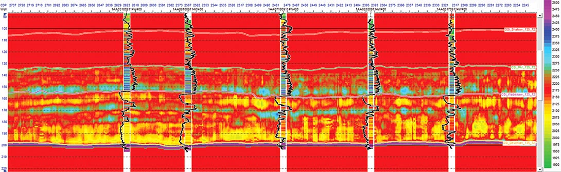
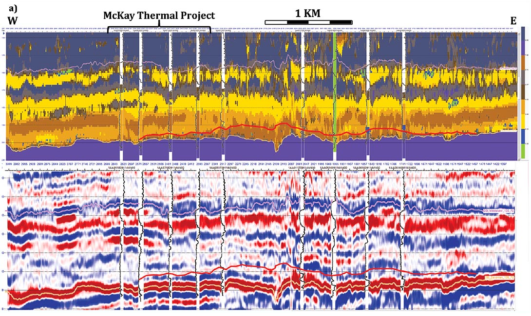
When we map these classes back to their location in space, we get the resulting classified seismic volume shown in Figure 14. The conventional seismic is shown at the same scale to contrast the relative comparison at the wells and usefulness of the products for betweenwell predictions.

Interpretation

We now have all the information we need to answer the original geological questions. But first the separate sand classes distinguished by the STAC QI need to be related to real life. This required a closer look at the core facies. Core facies that were initially subdivided based on presence and absence of burrows, matched closely to the QI facies when classified in terms of abundance and types of burrows. To quote the interpreter: ‘While we see more core facies than seismic facies, the fact that the same core facies were consistently classified into the same seismic facies was incredible. There is enough evidence to support the conclusion that the sedimentary structures impact the rock physics (the physical properties of the rock). ”

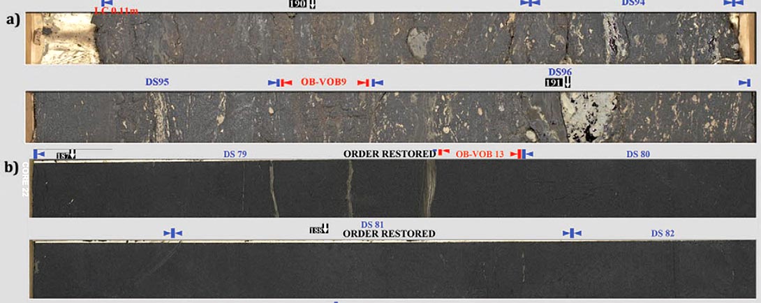
Figure 15 shows core photos of two facies types. In this case, the facies types are quite different but exhibit the same rock properties and fall into the same QI class (Sand 7) on the cross-plots. This might seem like a problem however the two facies are separated spatially and as shown on the classified seismic line in Figure 14, facies 7a represents the Middle McMurray which shows up at the base of the zone of interest (outlined in red) and facies 7b represents areas in the Upper McMurray.

Can facies variations and fluid types be distinguished using seismic data? Yes – with a systematic empirical approach followed by the comparison of geological definitions of facies to the seismic classes. Closing the loop in this fashion quantifies confidence in the final product.

Can inversion help resolve frustrating variations in seismic response at different wells where the geology was known to be consistent? Yes - the STAC QI classified facies volume shows the Wabiskaw sand and shale (where the problem was encountered) as consistent and continuous layers. While not determining the exact cause of the original issue this shows it to be a post-stackconventional- seismic-signal-averaging sort of problem that is avoided by using the STAC QI approach.

Can we distinguish the nature of the rocks that directly overlie the Devonian carbonates at the base of the reservoir zone? Yes – the facies volume clearly highlights variations in the rocks overlying the Devonian. The classification makes geological sense and will be tested with further drilling.

Conclusions

The MR 2D line inversion provided surprisingly accurate results, and allowed for matching to sedimentary facies that could not have been done with simple well ties between logs and conventional seismic. This was accomplished in spite of the imperfect or incomplete data. The McKay project was no different than any other in that sense and requires filling in the gaps with educated guesses and regional knowledge where data is lacking or suspect.

The STAC QI approach is not directed to answer specific geological questions in an isolated way. The process of discovering the geological ‘truth’ is systematic, integrated, and deterministic. The interpretation is done in the classification where questions can be addressed and sensitivities tested. The process is most effective when the geoscientists ‘close the loop’ by reconciling the apriori geological interpretation with the empirical evidence from the seismic QI.

This project was a feasibility study that demonstrated the effectiveness of the process and exceeded the initial expectations. Given the considerable cost of horizontal well pairs for steam injection and production in the oil sands the STAC QI results provide significant input into the geological understanding of the reservoir away from the existing wells. Investment in detailed reservoir understanding at this early stage of a development can provide the information required for informed and responsible ongoing reservoir management and monitoring.

Acknowledgements

The authors would like to thank Southern Pacific Resource Corp. for generous permission to publish these results. We would also like to acknowledge the specific contributions of Regan Kennedy at Earth Signal Processing Ltd., Chad Harris at Southern Pacific Resources Corp. and Neil Praught at Oil Sands Imaging Inc.