Introduction
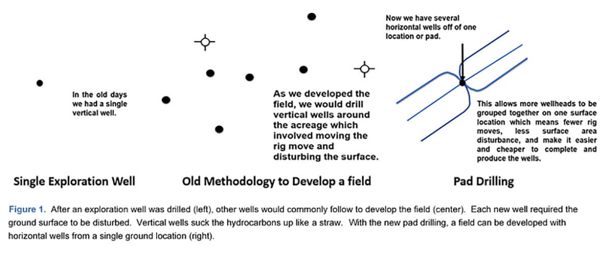
Horizontal wells and fracking are commonly used to increase hydrocarbon production while at the same time lowering the costs. This practice is helped by pad drilling, where multiple lateral horizontal wells can be drilled from a single location (Figure 1), reducing land use and cutting the need to move the rig.
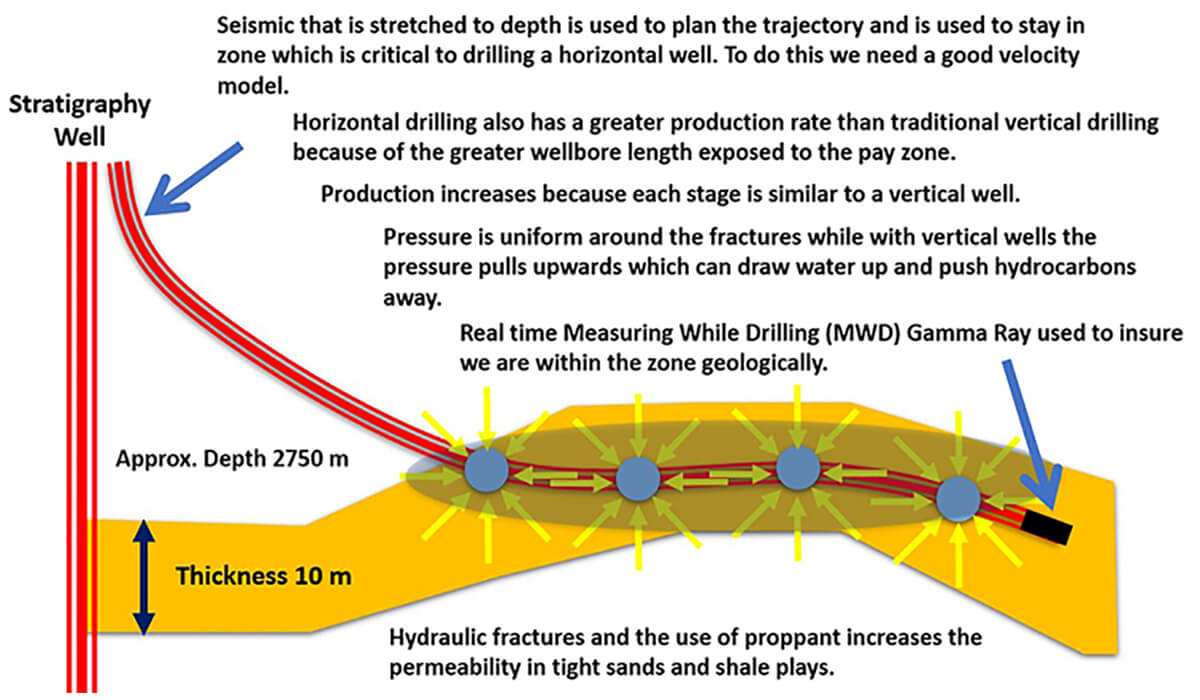
Horizontal wells are commonly fracked at intervals of 25 m. If a horizontal well is 2500 m long, this permits 100 frac stages where each stage acts almost as an independent well (Figure 2). Horizontal wells also have a better production rate than traditional vertical ones because of a greater wellbore length exposed to the pay zone. Besides, horizontal drilling avoids the problem with vertical wells where the pressure can draw water upwards and push away the hydrocarbons.
In planning horizontal wells, pre-existing fractures and faults need to be detected in advance. An unexpected fault can act as a thief, as the frac fluids and proppant may leak along the fault plane and away from the play interval. Occasionally, a fault may become reactivated and cause induced seismicity.
A fault with even a small displacement may cause the drill bit to suddenly exit the pay zone. If this happens, a decision is needed whether to correct by going up or down. The longer a horizontal well stays out of zone, the more production is lost. If the correction is made the wrong way, the losses can be large.
To detect possible faults, it is best to use an integrated, multidisciplinary approach bringing together:
- Seismic data
- Potential field data
- Surface and subsurface geology
The purpose of this paper is not to make every reader an expert in every relevant field of geoscience, but to let explorers and managers know what methods are available to detect subsurface faults and what questions to ask of the specialists they employ.
Seismic for fault detection
To image subtle faults reliably, seismic resolution needs to be high. Not all faults can be imaged successfully with seismic. Faults lacking appreciable vertical displacement may not be seen at all. Seismic reflection data are useful for detecting low-angle acoustic-impedance contrasts whereas faults tend to be steep, but that’s where potential–field methods and surface geology may help.
Vertical resolution in seismic surveys is 1/4λ (Widess, 1973) where λ = interval velocity / frequency = wavelength. Higher frequencies improve resolution, so thinner beds can be resolved. The smaller the sample rate, the higher the frequency that can be recorded and the thinner the bed that can be resolved. Therefore, some surveys use 1 ms sampling which has a Nyquist frequency of 500 Hz, so the field filter could be out – 450 Hz.
Problems can arise with inadequate sampling. An analogy is with pixels on a television screen, where a small number of large pixels will make the picture less refined and grainy. As the number of pixels is increased and the pixels get smaller, the resolution improves. Specific purposes of a seismic survey determine the data-acquisition parameters. Cooper (2004) developed a concept of trace density, where:

Where:
| Max Offset | = | Maximum offset at the zone of interest | |
| src line int | = | Source Line Interval | |
| rcvr line int | = | Receiver Line Interval | |
| rcvr int | = | Receiver Interval | |
| src int | = | Source Interval |
Increasing the trace density of 3D volumes improves subsurface imaging, which will improve well placement and field development (Lansley et al., 2007). Table 1 describes the ranges of trace density that can be required for different purposes (Cooper, 2004).
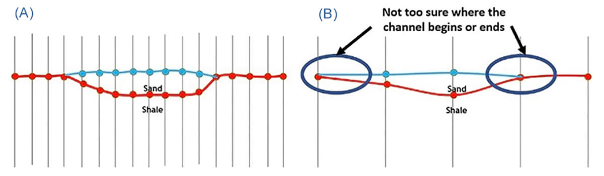
Figure 3 illustrates how a coarse bin size can lead to aliasing due to poor sampling horizontally. The channel is detected but its top, base and lateral extent are not resolved.
Horizontal resolution depends upon whether the data are migrated. With unmigrated data, the horizontal resolution is the migration aperture. There are three ways to calculate the migration aperture:
- Fresnel zone
- Diffraction energy
- Lateral displacement
| Trace Density | What the seismic is used for |
|---|---|
| Table 1. Table of trace density. | |
| 6000 – 18000 | Minimum of 6000 and this is good for very simple structure plays such as plains of Alberta data with good signal to noise ratio |
| 18000 – 25000 | For stratigraphic and sub-tuning plays with good signal to noise ratio |
| 25000 – 100000 | The trace density needs to be increased as the signal to noise ratio deteriorates, or as the structural complexity increases |
| 100000 – 1000000 | Used for poor signal to noise ratio or very complex structures like salt domes or foothills data |
| >1000000 | Used for 4D surveys and reservoir development |
Proper migration requires data across the entire migration aperture. When the data are migrated, it is as if the geophones are lowered through the earth until they are sitting on the reflector, at which time the migration aperture will have shrunk in 2D in one direction to λ/4 but will still extend its full width perpendicular to the line. With 3D data, the migration aperture is usefully shrunk in all directions to a small circle of λ/4.
Fresnel zone
The Fresnel zone is what’s referred to as the migration aperture. With a 2D or 3D seismic survey, the target needs to be completely covered by the migration aperture. The radius of the Fresnel zone is defined by:

Where:
| Velocity | = | RMS or stacking velocity | |
| t0 | = | Time of event | |
| frequency | = | Dominant frequency of the data at that time. | |
| 3500 | = | 783 |
(Equation from SEG Wiki [2019]).
Examples of Fresnel zone widths are presented in Table 2.
| Time (Seconds) | RMS Veloctiy (m/s) | Frequency (Hz) | Fresnel Zone (m) |
|---|---|---|---|
| Table 2. Fresnel Zone. | |||
| 1 | 1800 | 50 | 127 |
| 2 | 2000 | 40 | 224 |
| 3 | 3000 | 30 | 474 |
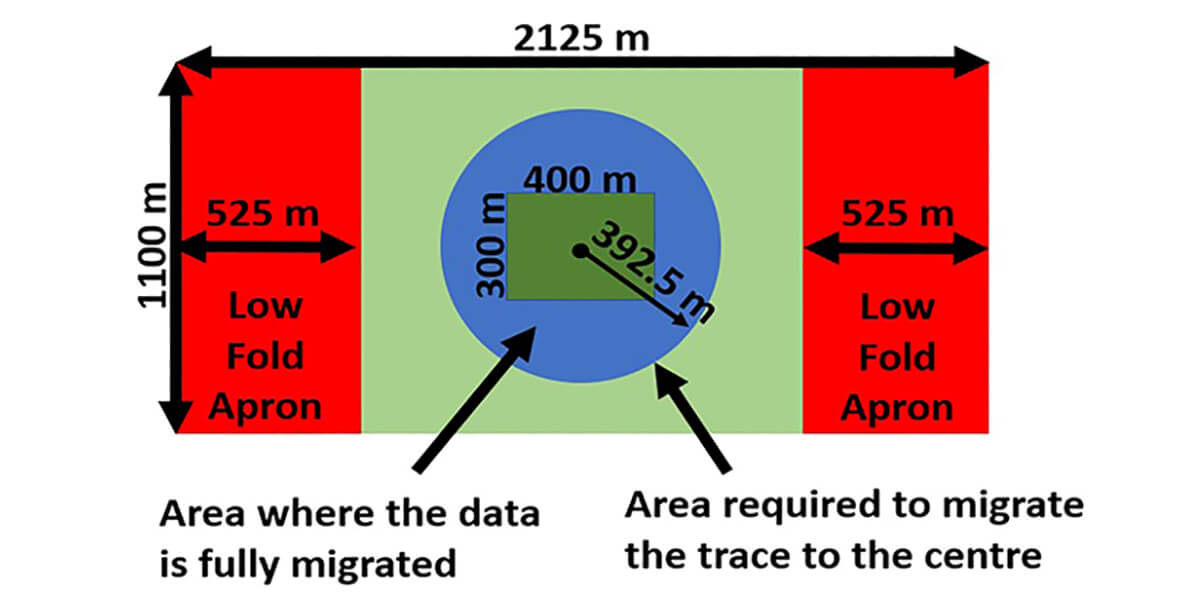
| 4 | 3500 | 20 | 783 |
If the Fresnel zone is 783 m (bottom row), for a Common Depth Point (CDP) to be properly imaged requires data in a radius of 392.5 m around the trace to enable migration (Figure 4). Without data within that radius, diffractions cannot be properly collapsed to a point.
After the data are migrated, the Fresnel zone collapses so that horizontal resolution is ¼ λ (Widess, 1973) where λ = interval velocity / frequency (as shown in Table 3).
| Time (Seconds) | RMS Veloctiy (m/s) | Frequency (Hz) | Fresnel Zone (m) |
|---|---|---|---|
| Table 3. Horizontal resolution after migration. | |||
| 1 | 1800 | 50 | 9 |
| 2 | 2000 | 40 | 3 |
| 3 | 3000 | 30 | 25 |
| 4 | 3500 | 20 | 44 |
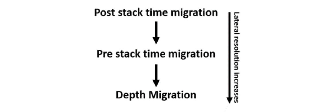
The type of migration also affects the horizontal resolution. Prestack time migration provides better resolution than post-stack time migration. Depth migration provides better resolution than prestack time migration (Figure 5).
Seismic frequency enhancements
Various ways exist to increase the frequency content of seismic data. One of the simplest is to use the near-offset stack which is generally a 0º -15º stack. The near offsets tend to be higher in frequency content and with fewer velocity errors.
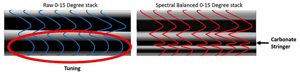
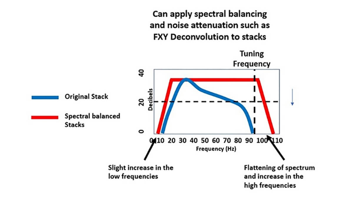
Spectral balancing
Spectral balancing boosts the frequencies to obtain better resolution (Figure 6). It especially boosts the low and high frequencies (Figure 7). Most spectral-balance programs balance the frequencies across narrow bands, and each frequency band is then equalized by its scaling function depending on the amplitude levels in this band (Chopra, 2011). All these scaled frequency bands are then added together to obtain the balanced sections. Testing is needed to make sure the frequency spectra are enhanced within a sensible bandwidth. Too much enhancement can cause undesirable ringing in the data.
Another way of enhancing the frequency spectrum is bluing, which is Colored Inversion applied to reflective stacked data. Bluing matches the seismic spectrum to the reflection log and by doing so produces a flat spectrum.
Spectral balancing brings out subtle events better than in the raw stack (Figure 6). Spectral balancing works best with the cleanest signal, and stacking helps to suppress random noise and enhance the signal. Spectral balancing will then flatten and broaden the frequency spectrum, which will increase both the vertical and horizontal resolution. FXY Deconvolution predicts linear events by making predictions in the frequency-space domain and is used after the spectral balancing for noise attenuation.
Many will argue that the vibrator data bandwidth is limited to the sweep frequency, but it needs to be recognized that the source wavelet is not identical to the sweep. This can be due to the vibrator’s base plate pressure being different from the sweep and imperfect coupling between the base plate and the earth (James, 2019). The harmonics also contain extra frequency components than the fundamental signal and this can broaden the bandwidth and enhance the S/N ratio (Hu et al., 2013). This means that the seismic bandwidth is not limited to the sweep frequency and may be higher.
The goal with the spectral balancing is to push the frequency above tuning. In eastern Alberta near the Alberta-Saskatchewan border there are thin sands such as the Sparky and McLaren sands in the Mannville and the frequency needs to be above the tuning frequency which is approximately 95 Hz to image these sands within the seismic. While in the deep basin the goal is to bring out the thin tight channel sands or brittle stringers within the shales to target for horizontal drilling.
Acoustic inversion
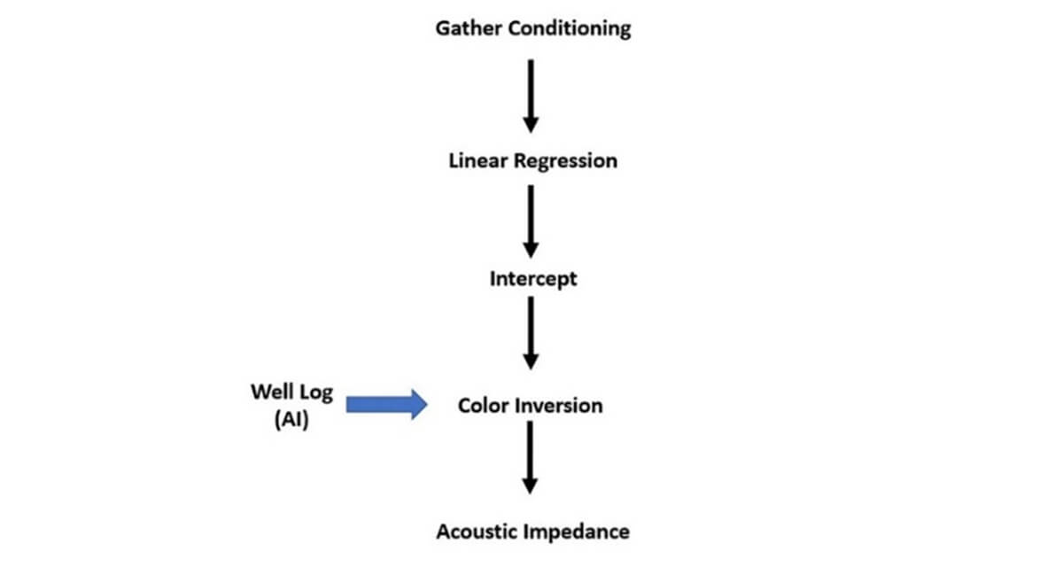
Acoustic impedance is the inversion or -90° phase rotation or color inversion of the zero-offset stack or intercept, which is calculated using linear regression of amplitude points. Traditionally, the amplitude at different offsets/angles within the full gather is used for the linear regression to calculate the intercept and gradient, but a new process uses angle gathers created from FXY Decon - spectral whitened - angle stacks.
Stacking is one of the most powerful noise attenuation programs available in processing and AVO can be captured within the partial stacks or angle stacks. The three angle stacks that will be used are: 7.5o (0o to 15o); 22.5o (15o to 30o); and 37.5o (30o to 45o) and spectral whitening attempts to remove the time-dependent loss of high frequencies in the data due to attenuation (Cary, 2006). It also allows the frequencies to be enhanced so that the data are “detuned” and a better zero-offset stack or intercept is created. Detuning is increasing the frequency so that it eliminates tuning of the wavelet between thin beds.
The workflow to create acoustic impedance is shown in Figure 8.
Colored inversion
Colored inversion (Lancaster & Whitcombe, 2000; Connolly, 2010) is the process to create band-limited impedance, which has a power-law spectrum limited by the bandwidth (Connolly, 2010). This process will result in optimal resolution within a given bandwidth. Colored inversion should be run on the zero offset stack to match it with the spectrum of the acoustic impedance well log to enhance the frequencies. With deterministic inversion, the model is created by interpolating filtered well-log values along seismic horizons. With channels, mis-picks (Figure 9) can cause the model to leak into the inversion. For quality control, a colored inversion can be useful since colored inversion does not use a model and it can show where the well model may have leaked through.

If the seismic data are recorded so that low frequencies are enhanced by using a non-linear vibrator sweep that ranges from 3 to 100 Hz along with low-frequency geophones (3 Hz), then a relative inversion such as color inversion will approximate a deterministic inversion, and trends will be visible in the data. The trends come from the low frequencies in the inverted data.
Deterministic inversion improves the resolution by removing the wavelet. The wavelet can change with traveltime, and there can be errors in how the wavelet is calculated. Colored inversion relies on matching the seismic spectrum to the well-log spectrum to increase resolution.
Structural smoothing
Structural smoothing aims to remove noise, but it preserves and even highlights relevant details such as those due to structural and stratigraphic discontinuities. Thus, colored inverted acoustic impedance can reveal subtle faults
Information from structural smoothed color inverted acoustic impedance can then become input for structural attributes such as spectral decomposition, coherency, curvature and semblance analysis, all of which can reveal subtle faults not initially seen in the seismic data.
Geometric attributes and automatic fault detection
Geometric attributes such as coherency, curvature and flexure look at changes in the seismic caused by variation in structure, stratigraphy, lithology, porosity, and structural discontinuities such as fractures or faults. The structural smoothed color-inverted acoustic impedance volume can help highlight discontinuities. A subsequent run of coherency, curvature and flexure can further illuminate faults and fractures in the seismic data.
Coherency measures the similarity between waveforms or traces. Geologically, a highly coherent seismic waveform indicates continuous lateral lithology. An abrupt change in the waveform might indicate a fault or a fracture.
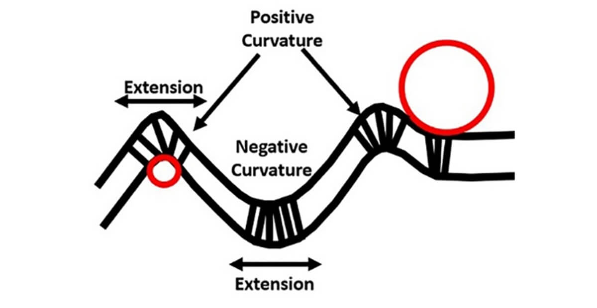
Another common geometric attribute for fault detection is curvature. Curvature defines how bent a curve is at a given point on the curve. The curvature attribute is a surface-related attribute which helps to bring out faults, fractures, flexures and folds.
There are two different types of curvature:
- Horizon curvature utilizes picked horizons. On the downside, horizon curvature is affected by how the horizons were picked in noisy seismic data that are contaminated with the acquisition footprint, or how horizons are picked through areas lacking consistent impedance contrasts.
- Volumetric curvature is calculated from a vertical window of seismic samples and is statistically less sensitive to noise. It alleviates the need for picking horizons in regions where no continuous surface exists.
With volumetric curvature, for example, the most-positive curvature can define the flanks of channels, potential levees, and overbank deposits. This can occur due to differential compaction or the presence of levees, while the most-negative curvature can highlight the channel axes, as shown in Figure 10.
Curvatures can sometimes be used to predict high fracture intensity in the crest-forelimb parts of a fold, where fractures tend to be concentrated, as is known from outcrop mapping (Di and Gao, 2016). Curvature can also highlight fault offsets, such as with raised and downthrown fault blocks, but it does not detect faults directly (Di and Gao, 2016).
Seismic flexure is used to evaluate the lateral changes in the curvature of a seismic event (Gao, 2013; Yu, 2014; Di and Gao, 2016) and so a fault is highlighted as a lineament (Di and Gao, 2016). Flexure is considered the most useful when extracted perpendicular to the orientation of the dominant deformation trend. It offers useful insights into the qualitative and quantitative fracture characteristics (Di and Gao, 2016). For example:
- Magnitude indicates the intensity of faulting and fracturing;
- Azimuth defines the orientation of most-likely fracture trends;
- Sign differentiates the sense of displacement of faults.
Some interpretation packages use seismic attributes to automatically pick faults. This, however, depends on pre-selected parameters, so false picks can result while other faults can be missed. In the end, human oversight and double-checking are essential.
Not all faults and fractures can be detected in seismic data, and other information needs to be used, such as potential fields and surface geology. No particular methodology replaces any other. The more information, the better. All these methods are mutually complementary.
Potential-field geophysical methods for fault detection
Gravity and magnetic methods are of great value in the detection of faults and fractures. In the mining industry, potential-field methods are used for this purpose very commonly on a prospect scale. We encourage this near-universal mining experience to be used also in oil and gas development.
Gravity and magnetic methods do not replace seismic but add to it. Despite being comparatively low-resolution, they have some very big advantages.
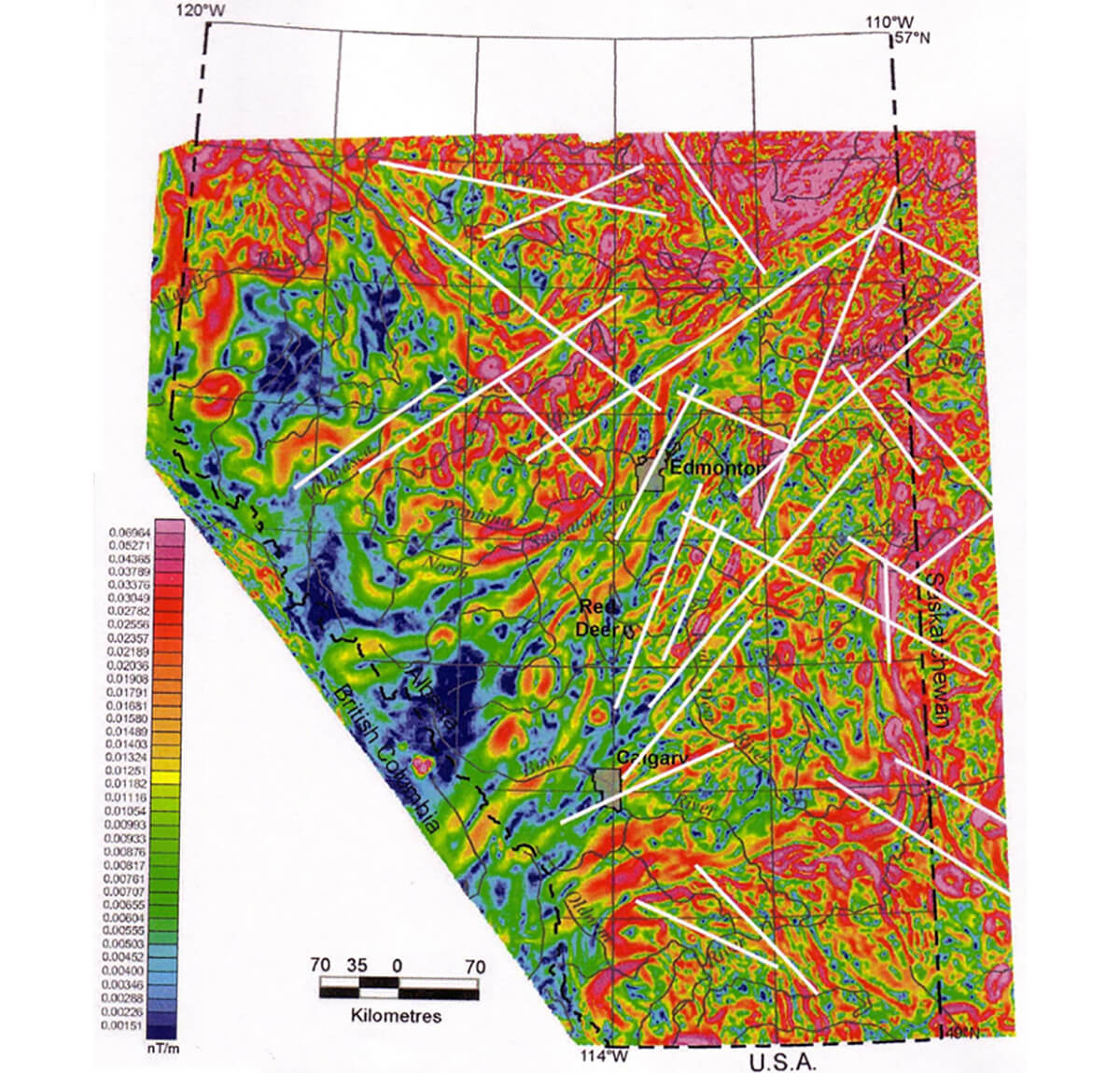
These geophysical methods passively measure natural variations in the Earth’s gravity and magnetic fields over a wide or local map area (Figures 11 and 12). Interpreters then try to relate these variations to geologic features in the subsurface (e.g., Nettleton, 1971; Telford et al., 1976; Hinze, ed., 1985; Goodacre, org., 1986; Lyatsky et al., 2005). Lacking a controlled source, such surveys can have a low environmental footprint, and they do not disrupt ground operations such as farming.
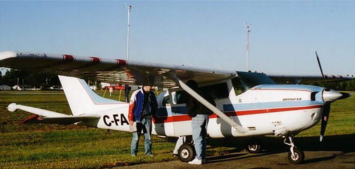

At a comparatively low cost, airborne potential-field surveys can provide coverage of large and small areas. Allowing quick regional coverage, even gravity surveys can now be recorded from an aircraft with fairly high reliability. Ground and helicopter-borne surveys could be appropriate in local work; the use of drones in geophysical surveys is in its infancy but spreading. Gradient surveys can help to detect shallow and subtle anomalies in local studies.
In Canada, digital regional gravity and magnetic data are available at zero cost from federal government agencies. Commonly, government gravity data are too sparse for very localized work (roughly, just one ground station per township in the Canadian Prairies) but the magnetic data were usually flown with a half-mile line spacing or tighter. Still, even sparse gravity data can give a general idea of faults that might be crossing a prospect area, and a half-mile flight-line spacing might be sufficient to adequately sample the basement-sourced anomalies in most of the Alberta Basin (Lyatsky et al., 2005). Local and detailed surveys are commonly acquired by oil and mining companies.
How to make geological sense of geophysical anomalies
The physical rock property that links gravity anomalies to rock composition is bulk density. The rock property that links magnetic anomalies to rock composition is total magnetization. Thus, each potential-field method valuably provides its own picture of the subsurface. These methods are complementary and not mutually redundant.
Density is a scalar: it has no direction. Magnetization is a vector total of a vast and commonly unresolvable variety of remanent and induced magnetizations of innumerable types and vintages. Deceptively, and unlike bulk density, magnetization can depend on tiny variations in the occurrence and distribution of some particular minerals which may have little relation to the overall lithology.
A geophysical anomaly is the difference between the observed (measured) geophysical-field value and the value that would be observed at the same location and time if the earth were more uniform than it is (Lyatsky, 2004). Non-uniformities in the physical properties of rocks give rise to geophysical anomalies.
Being responsive to lateral variations in rock properties, gravity and magnetic methods are best suited for detecting steep discontinuities such as faults. Seismic reflection methods, by contrast, are usually better suited for finding vertical rock variations and low-angle discontinuities such as layer boundaries.
The gravity field is simple, unipolar and almost perfectly vertical. The geomagnetic field is complicated: it has two or more poles and it is commonly strongly non-vertical. Besides, it changes all the time (causing rapid migration of the magnetic poles), necessitating frequent updates by government agencies.
Gravity lows (negative anomalies) occur where rocks in the subsurface have a comparatively low density, which reduces their downward gravitational pull. Where the rock density underfoot is relatively high, the gravitational pull is increased and a gravity high (positive anomaly) occurs.
Magnetic anomalies are more complicated and harder to interpret, because the magnetic field and rock magnetization are both very complicated. With a non-vertical, dipolar field, a single rock-made anomaly source can be deceptively associated with a pair of anomalies: a high and a low side by side.
Gravity and magnetic surveys should be designed purposefully, to resolve at minimum cost the specific kind of anomalies that are expected from the geologic targets of interest. Make a survey too tight, and money is wasted on redundant coverage. Make it too sparse, and the desirable anomalies are under-sampled and not delineated in enough detail (as also in seismic: Figure 3). Optimally, you design the sparsest and smallest – and hence the cheapest – survey that would resolve all the expected desirable anomalies.
Examples of exploration use
In the platformal, Phanerozoic Alberta and Williston basins in western Canada, most big magnetic and gravity anomalies are associated with ductile structures and rock-composition variations in the crystalline basement that were inherited from orogenic events in the Precambrian. Such ductile, ancient structures were seldom reactivated, and they had relatively little influence on the Phanerozoic basins above.
More important for exploration are the later, brittle basement faults and fractures, whose vertical offset if any can be as little as a few meters, sometimes below seismic resolution.
Such brittle faults had a variety of direct and indirect influences on many intervals in the Phanerozoic sedimentary cover. They are sometimes associated with subtle gravity and magnetic lineaments, some of which cut across the regional pattern of major anomalies. To help delineate fault networks, a public-domain, regional gravity and magnetic atlas of the southern and central part of the Alberta Basin was created by the Alberta Geological Survey (Lyatsky et al., 2005).
Two of us (Lyatsky and Bridge) have previously used gravity and magnetic data in oil-exploration settings to delineate fracture and fault networks on a much smaller scale. These studies are proprietary, but our approach to data processing and interpretation was similar the one in the AGS atlas.
A gravity or magnetic lineament can be a gradient zone, a linear break in the anomaly pattern, a straight anomaly, or even an alignment of separate local anomalies (Figure 13). Long lineaments are more likely to be associated with faults than short ones, especially if they occur in swarms or belong to a recurring regional pattern. Lineaments are best picked on a plotted paper map by hand, by looking at the map at a low angle on a table and slowly rotating it to change your viewing azimuth. As in the old days, a trained eye and some crayons work well!
The best data-processing methods are simple and intuitive, so that derivative maps and anomalies are easy to relate to their precursors in the raw data. Because it can be hard to know in advance which processing methods and parameters will deliver the most geologically useful results, a great deal of experimentation might be required to achieve the most useful derivative-map selection. Plotting maps with a combination of color coding and line contours (unless the map is too busy for contours) can produce a very vivid depiction of anomalies.
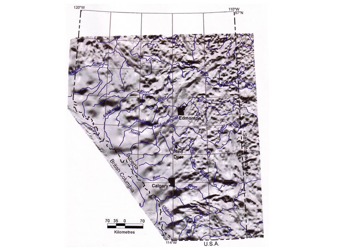
Gravity and magnetic data can be processed specifically to highlight subtle lineaments. Particularly useful processing methods tend to be first and second horizontal and vertical derivatives, third-order residuals, automatic gain control, total gradient (analytic signal) and shaded-relief maps (or shadowgrams: Figure 14). Because shadowgrams can act as directional filters based on the “sun” azimuth, a large suite of them could be required with many different azimuths and inclinations.
Reduction to pole assumes that all magnetization is induced and remanence is absent. Such situations are in fact uncommon and should not be assumed without examining the anomaly causing-rocks, so pole reduction is not advisable as a default. Wavelength filtering has a major pitfall such as Gibbs ringing that on a 2-D map can produce lineament-like artifacts, and a smaller question of arbitrarily chosen cut-offs, so it is best avoided.
To help identify faults, gravity and magnetic lineaments should be compared with topographic and drainage lineaments. Seismic data and geological studies can help to determine if suspected faults had an influence, primary or secondary, on any play interval.
Surface geology for fault detection
Drainage lineaments
Surficial lineaments can be valuable in the detection of fractures, joints and faults, and they deserve to be examined much more commonly in the petroleum industry. Many remotely sensed lineaments are surface manifestations of regional fractures and deep-seated faults (e.g., Mollard, 1988).
A lineament is a mappable linear or curvilinear surface feature. Current technologies, such as LiDAR and satellite imaging, provide excellent methods for identifying linear surficial features, especially linear drainage patterns, that can be related to subsurface features such as joints and faults.
Drainage lineaments in topographic maps may vary from small and intermittent creeks to large rivers. Small-scale and large-scale drainage patterns are largely influenced by slope, lithology, and bedrock composition and structure. Observation of slope and drainage patterns can discern lineaments that are most likely to be related to subsurface structures.
Topographic maps
Canadian topographic series maps at 1:50,000 are an excellent, readily available and low-cost medium for observing drainage lineaments. They provide a satisfactory scale and resolution of imagery for local and regional lineament selection, where lineaments sometimes group into parallel to subparallel sets correlating with subsurface joints, and longer lineaments could be correlated with faults.
Fault-related surface lineaments can be parallel or transverse to the joint sets. Subtle lineament features like tonal variations in imagery and patterns of vegetation are not seen in topographic maps and are not necessary for bedrock structural determination; they may be cultural (man-made) and not geologic. Topographic maps are generally more effective that aerial photos for identifying drainage lineaments because topographic maps do not show the multitude of cultural linear features such as agricultural practices, vegetation boundaries, roads, cutlines, bush trails etc.
Regions with very low relief will not easily produce recognizable drainage lineaments that can be observed on topographic maps. As with gravity and magnetic maps, shaded-relief images of high-resolution LiDAR digital elevation models can be used to capture the subtle lineaments that may occur in very low-relief regions.
Overburden cover
Most of the western Canada plains have an overburden that is relatively uniform on a regional scale. Consequently, it is optimal for the observation of drainage lineaments that are directly related to subsurface structures.
Overburden-covered regions with a predominance of clay till in the upper portion of the Quaternary cover are the terrain most suitable for topographic-lineament interpretation. Clay tills are ideal for developing joint sets and depressions along faults that are expressed at the surface as minor or major linear drainage features. Joints commonly provide paths of weakness along which surface drainage preferentially develops.
Sandy to gravelly surficial overburden tends to be a poor medium for transmitting subsurface features to the surface because of the unconsolidated nature of the materials. Physiographic glacial features such as drumlins and dune sands can even mask subsurface structures.
Topographic maps capture most features required for identifying subsurface joints and faults, but LiDAR interpretation is probably the most suitable method for identifying lineaments in regions of outcrop, sub-outcrop and shallow overburden.
Relation of surficial lineaments to basement structure
Small-scale movements on basement faults, or groundwater channeling and weathering along basement faults under partially or recently lithified sedimentary cover, can create joints. These joints sometimes form parallel or subparallel rectilinear sets that cover large areas and are often related to underlying basement faults. Since the Quaternary cover in the western Canadian plains is essentially undeformed, the joint sets reflect both compaction jointing and the original basement faults and fractures. However, joints and joint patterns can be influenced both by inhomogeneities in the sedimentary section and later stresses in the sedimentary cover such as those due to salt dissolution and collapse (although salt-dissolution fronts can themselves be influenced by fluid-conducting deeper fractures).
Regional orthogonal joint sets occur in Precambrian rocks exposed in northeastern Alberta (Langenberg, 1983). These joint sets have been described across the Athabasca oil-sands region (Babcock and Sheldon, 1979) and through central and southern Alberta (Babcock, 1973, 1974), occurring in the Phanerozoic sedimentary rocks and Quaternary cover. The orthogonal joint sets are believed to be caused by recurrence of similar stress fields affecting the Precambrian basement and the Phanerozoic cover, or by reactivation of established brittle joints and faults.
Two major lineament sets, one trending northeast and one northwest, occur throughout Western Canadian Sedimentary Basin region. Misra et al. (1991) interpreted these lineaments to represent nearly vertical, tensional stress faults in the Phanerozoic sedimentary rocks. Fracture sets that outline basement fault blocks are interpreted to control the orientation of faults in the sedimentary cover and the orientation of surficial lineaments. Basement fault zones appear as broad surficial lineament zones, and higher lineament densities around major arches in the basin are interpreted to indicate increased stresses in the basement rocks.
There are numerous examples in the international literature where mapping of drainage lineaments by simple or sophisticated methods reveals a good correlation between drainage lineaments and basement structures. Drainage lineaments in Late Pleistocene and Holocene cover in southeastern Louisiana, for example, are related to the mapped joint pattern in underlying Mesozoic and Cenozoic strata, indicating that the trends of physiographic lineaments are controlled by deeper structure (Birdseye et al., 1988).
A study in north-central Louisiana compared deep dipmeter records to drainage lineaments (McCulloh, 2008). Dip angles of 20° or more were treated as reflecting structure, as opposed to those less than 20° which were treated as depositional in origin. Remarkably, straight drainage lineaments over 300 m in length showed three distinct trends that had no statistically significant difference from the examined dipmeter population with dip angles exceeding 20°.
Picking and classifying lineaments
As with gravity and magnetic lineaments, a major challenge in picking surficial lineaments is that the most practical way to pick them is manually. Manual picking can be subjective and influenced by personal bias, but automatic picks rely too much on pre-selected arbitrary parameters.
Topographic maps at a 1:50,000 scale provide a good resolution of imagery for picking drainage lineaments except in regions of very low relief. Lineaments are commonly classified or ranked based on their length and orientation. They can also be classified based on their degree of linearity or frequency of minor offsets on the lineation.
Conclusion
Enhancement of seismic data can significantly improve resolution and our ability to detect subtle faults ahead of drilling. Gravity and magnetic data can provide their own picture of fault and fracture patterns. Still, not all faults or fractures can be seen with seismic and potential-field data, and surface geology needs to be integrated to provide a more complete picture. Besides, any subsurface information from existing wells (Figure 15) should also be utilized.
Brittle, high-angle faults and fractures can have a variety of direct and indirect geologic influences on many intervals in the sedimentary cover. They are commonly associated with subtle gravity and magnetic lineaments, some of which cut across the regional pattern of major anomalies.
Potential-field and seismic data should be compared to what is seen in topographic maps. These maps capture many features required for identifying joints and faults, but LiDAR interpretation is also an excellent method for identifying lineaments in regions of outcrop, sub-outcrop and shallow overburden. Seismic, potential-field data, and surficial-lineament information can be included into a common geomodel.
Understanding the faults ahead of drilling can prevent errors and avoid induced seismicity, saving both money and corporate reputations. We strongly encourage exploration and development managers to make use of all available methods that can help with fault and fracture detection, and to include in their teams an appropriately wide spectrum of geoscience expertise.


Join the Conversation
Interested in starting, or contributing to a conversation about an article or issue of the RECORDER? Join our CSEG LinkedIn Group.
Share This Article