Microseismic, 3D and 4D Applications and its Relation to Geomechanics and Completion Performance

Summary

This study demonstrates empirical relationships derived from microseismic, 3D inversion attributes and 4D seismic to production in unconventional shale in the Horn River Basin. Production variations are explained through the use of the above mentioned tools and a careful investigation of stimulated rock volume. These production variations are shown to occur from a highly stressed zone influenced by a fault which intersects the north portion of a well pad. Estimates of stimulated rock volume are driven by the microsesmic event locations and the 4D response. It is shown that high b-values occurred in brittle rock and in a lower stress regime and low b-value stages occur in ductile rock in a relatively higher stress regime.

Introduction

For unconventional resource plays the spatial extent of hydraulic fracturing and resulting stimulated rock volume (SRV) is often unknown. Identifying stimulation success or failure is a necessity to increase production through improved pad placement and well spacing. Microseismic data is one of the few tools available to interpret completions effectiveness and the extent of the stimulated volume. Initial interpretations of microseismic data involve estimating fracture dimensions such as half lengths and vertical height growth or fitting a cloud to the cluster of events. This method of interpretation can have large spatial errors due to uncertainties in microseismic event locations which lead to uncertain fracture dimensions and estimates of SRV. To quantify the effectiveness of stimulation, the bvalue method is used and mapped spatially to identify variations. The b-value is calculated using the recorded magnitude of the individual events and thus to some extent is independent of event location and the associated location error. This analysis is used to infer in-situ stress information and rock quality at the stage level, which gives new insights into the stimulation beyond event location interpretation. b-values are also correlated to inverted seismic volumes, so that the rock quality that is being fractured is evaluated and this can be used to aid future well pad planning. Finally, using time lapse seismic over the stimulated zone, the 4D response is interpreted for SRV from the pre and post frack differences.

The case study used to demonstrate the correlations between microseismic and rock properties is an unconventional shale play in the Horn River Basin in North East BC. The Horn River Basin consists of the Muskwa, Otter Park and Evie shale’s which lie above the Keg River carbonate. The Horn River shale was thought to be relatively homogeneous throughout the basin but with an increase in drilling, completions and production in the basin, it is apparent that the basin is more heterogeneous than first thought (Close et al., 2012). The well pad analyzed in this study is an example of the heterogeneity as it had production variations where the northern portion of the pad (north pad) had reduced EUR relative to the southern portion of the pad (south pad). The cause of the EUR variations over the pad is investigated.

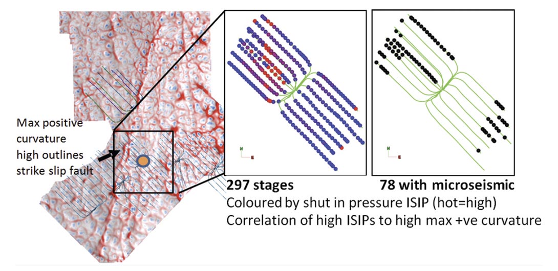
During completions, anomalously high instantaneous shut in pressures (ISIP) were recorded over the north pad. The locations of these stages qualitatively correlate with an extensive (positive curvature high) fault on reflection seismic data (Figure 1). The high ISIP’s combined with the fault that intersects the entire north pad is hypothesized to have affected the production on the north pad. In an attempt to estimate SRV from completions and to estimate in-situ rock properties, a vertical downhole microseismic survey was acquired to understand the production variations independently of reflection seismic attributes. In total approximately 300 stages were completed, and of those, 78 recorded microseismic with approximately 15000 located events. The majority of the recorded stages were at the toes of the pads. In addition, two wells were recorded from toe to heel on the north pad.

3D Seismic Inversion Attributes

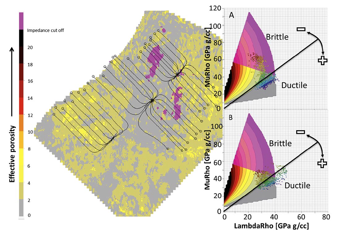
The microseimsic data was compared to the inverted seismic attributes LambdaRho and MuRho (Figure 2). Templates have been created to interpret seismic data in LambdaRho-MuRho space (LMR) (Perez et al., 2010, 2011 and Goodway et al., 2006, 2010) to understand the variation in rock properties in seismic data. Fundamental conclusions which apply to shale completions from these templates are the location of brittle vs ductile rock in LMR space (Figure 2) and the closure stress scalar given by the isotropic closure stress equation (Goodway et al., 2006, 2010).

The closure stress scalar relates the effective minimum horizontal closure stress ( δ_zz – p ) to the overburden stress ( δ_xx – p ). The closure stress scalar is equal to the slope of a straight line through the origin in LMR space where an increase in closure stress scalar (decreased slope in LMR) implies an increase in pressure required to sustain hydraulic fracturing (Close et al., 2012).

Figure 2 shows the zone of interest where, east of the fault a zone is interpreted to be ductile rock under relatively higher closure stress. This is consistent with the expected result for isotropic inversion of anisotropic data corresponding to the values within the P impedance cut off (pink zone). The south pad is located in primarily brittle rock under relatively lower closure stress interpreted from the lower Lambda-rho values. This implies that the north wells have been placed in rock within a zone of increased stress interpreted from the higher closure stress scalar values (slope in LMR space) and hydraulic fracturing will have to overcome this to fracture the rock.

Microseismic

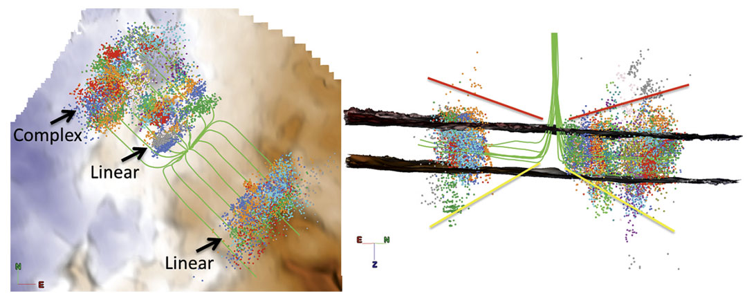
The microseimic results are displayed in Figure 3 in map and cross section view. As distance from the recording wells increases, there is an increase in event location error due to the difficulty in picking P and S wave arrival times resulting from the reduction of amplitudes. This error is qualitatively shown by the red and yellow lines where the red line represents low velocity shale while the yellow line is a high velocity carbonate. In map view, the south pad events are relatively linear, aligned parallel to the direction of maximum horizontal stress. In comparison, the north pad microseismic activity at the toe stages is complex with no apparent preferred orientation. Towards the heel of the north pad, the microseismic events become linear and parallel to the direction of maximum horizontal stress. The cross section view displays this transition from complex to linear event clusters as the stages go from the toe to heel over the north pad. There is a decrease in microseismic event density in the central portion of the north pad which separates the zones of complex and linear clouds. The sub-optimal completions inferred from the complex and varying nature of the microsesimc activity along the well may explain the reduced production over the north pad. In the south pad the stages appear to be linear with little complexity and the production from these wells are within an expected range.

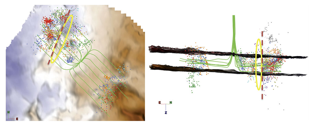
In an attempt to interpret the event cluster variations over the north pad with increased confidence, a moment magnitude cutoff of -1.8 is used to display events (Figure 4). The cross section view of Figure 4 shows a gap in microseismic activity that was noted as a decrease in event density (Figure 3). The microseismic activity from stages located in the gap is deflected towards the previously fractured toe of the well. This activity gap begins in very close proximity to the previously noted fault, which crosses the north pad (Figure 1), and to the ductile high closure stress zone interpreted from LMR crossplot (Figure 2). The events appear to have traveled west and vertically, refracking previous zones and understimulating the zone east of the fault. Higher magnitude events appear to cluster in close proximity to the fault, interpreted as stages within the high closure stress zone. The stages were unsuccessful at fracturing the highly stressed rock east of the fault and thus found a lower stress pathway back towards the toe of the stages which resulted in reduced SRV over the north pad. To further analyze and understand the stress variations that are affecting the microseismic locations, the b-value method is utilized.

b-value method

To investigate and explain microseismic variations, b-value analysis is employed. Gutenberg and Richter (1954) observed a linear relationship between earthquake magnitudes and the frequency at which they occur. This relationship is given by the frequency magnitude distribution equation (FMD)

where N(M) is the number of events greater than or equal to magnitude M and b is the slope which relates the log of the frequency to the magnitude of the event. The method used to estimate the b-value was the maximum likelihood method (Aki, 1965 and Bender, 1983) given by

where M is the mean magnitude, M_C is the magnitude of completeness and ΔM_bin is the width of the magnitude bin used. The magnitude of completeness is the theoretical value at which all seismic events above or equal to this magnitude have been recorded and above this magnitude the FMD becomes linear (Wiemer and Wyss, 2000). From equation (3) it is apparent that the accuracy of the magnitude of completeness estimation will impact the b-value. For this study, the maximum curvature (MAXC) method was used to calculate the magnitude of completeness. The MAXC method calculates M_C as being the magnitude at which the FMD has maximum curvature, or the magnitude value which is equal to the magnitude bin with the largest number of events in the non-cumulative FMD. However this method has been shown to consistently underestimate the magnitude of completeness which would allow events from the nonlinear portion of the FMD to be used in the b-value calculation. Overcoming this limitation is achieved by applying an additional constant after calculating MC using the MAXC method (Woessner and Wiemer, 2005). There is a compromise to ensure that the magnitude of completeness has been met and maximizing the number of events used in the b-value calculation. As suggested from the noted underestimation of M_C, 0.2 was added to the calculated M_C optimizing both the number of events in the calculation and ensuring the magnitude of completeness has been reached.

The b-value uncertainty was estimated using the equation by Shi and Bolt (1982) given by

where M is the mean magnitude and N is the number of events. b-values were only calculated on stages where the number of events exceeded 30 to ensure an acceptable sample size for the calculation. From experimental observation, several b-value relationships have been established which can assist in interpreting gas shale completions.

1. b-values are inversely proportional to stress (Amitrano, 2003 and Urbancic, 1992).
2. b-values are related to the brittle/ductile nature of the rock where, in general, more ductile rock have lower b-values and brittle rock have higher b-values (Amitrano, 2003).

Applying these relationships to shale completions, high b-values occur in brittle rock under relatively low stress where low bvalues occur in more ductile rock under high stress. In general bvalues for hydraulic stimulation are ≈2 while those associated with natural faults are ≈1 (Maxwell et al., 2009). With these relationships, information can be extracted from microseismic data beyond event locations that give insights to the in-situ fractured rock and stress state.

b-value analysis

The pad has a total of 78 stages that recorded microseismic data. Of these stages, 52 met the minimum event number for b-value estimation (Figure 5). Of the 52 stages, 37 were on the north pad and 15 on the south pad. The average b-values across the north and south pad were ≈1.57 and ≈1.96 respectively. The north and south average b-values are interpreted to be within the approximate value for hydraulic fracturing (≈2). These lower b-values are not interpreted as an indication of fault activation as the low values occur across the entire north pad and have b-values above the approximate value to imply fault activation (≈1). There is no microseismic evidence of linear activity near the fault and the magnitudes recorded over the entire pad were small relative to fault activation magnitudes.

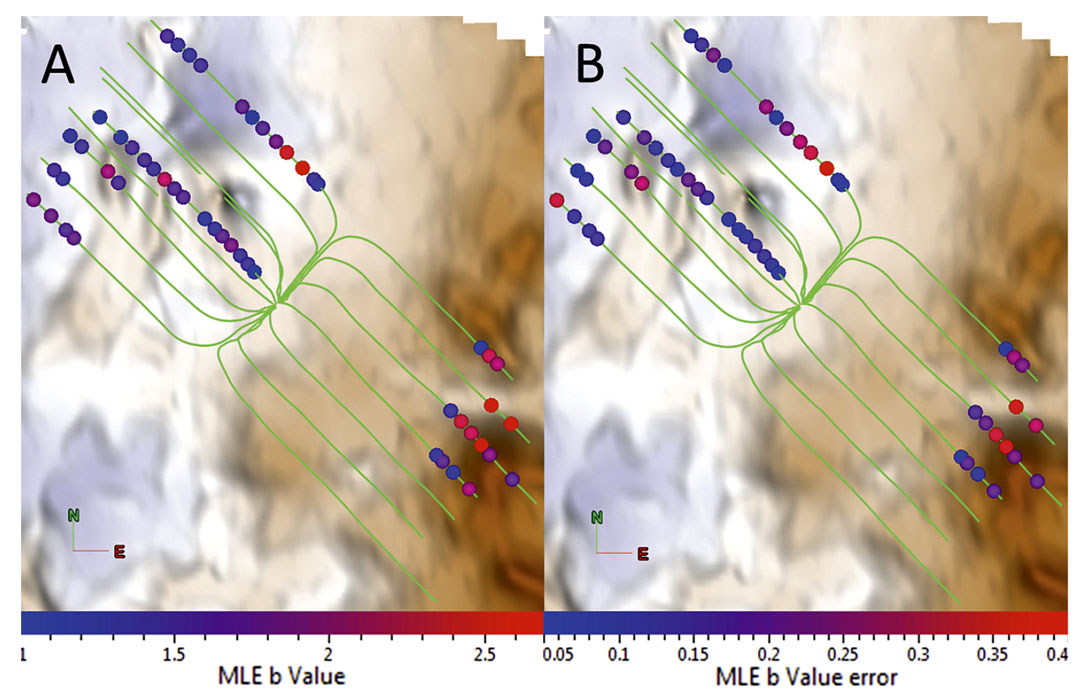
The low b-value over the north pad is interpreted as having relatively higher in-situ stress compared to the south pad caused by the fault. In contrast, the south pad is under a stress regime that permits the stages to achieve a b-value of ≈2 which is the average for hydraulic fracturing. This interpretation agrees with the high ISIP’s and the LMR analysis (Figures 1 and 2).

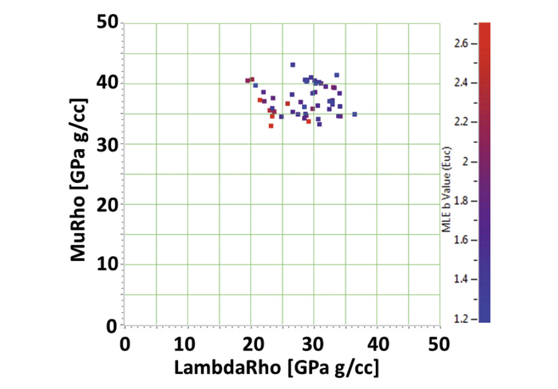
To further analyze the b-values obtained, a comparison was made to the seismic inversion attributes LambdaRho and MuRho. Figure 6 displays a cross-plot of averaged LMR values extracted along the wellbore at the stage locations colored by bvalue. In the LMR crossplot, there is an inversely proportional trend between LambdaRho and b-value. The stages with high bvalues occur in low LambdaRho regions where the rock is more brittle and has lower closure stress (Figure 2) compared to the stages which have low b-values. This LMR cross-plot, colored by b-values suggests that the LMR templates can predict zones of brittle rock under low closure stress and ductile zones under high closure stress as confirmed by the high and low b-values.

4D Survey

At the time of the monitor survey, approximately 100 stages had been completed. Within those 100 stages, four wells were completed toe to heel on the north pad as well as all the microseismic stages. The monitor survey was recorded during completions and this lead to high noise levels at the pad center. The 4D seismic response resulting from hydraulic stimulation is expected to originate from two main sources.

1. Increase in fracture density caused by fracking.
2. Influence of the unrecovered frack fluid and proppant placed into the dry gas shale, as the post completion monitor survey was acquired during pumping and prior to production.

The 4D response from the two sources alter the impedance of the stimulated zone in opposing ways. In general, an increase in fracture density will decrease the P-impedance, whereas a fluid substitution from dry to wet and the addition of quartz to the rock volume increase the P-impedance. The 4D response shows a noticeable amplitude and isochron difference with the greatest change at the toe of the wells. This shows that hydraulic fracturing alters the rock properties sufficiently and a 4D response can be interpreted from a pre and post frack survey.

4D Amplitude and Isochron Analysis

The schematic in Figure 7 displays the expected 4D response as a slight time delay between the monitor and baseline surveys. The result is a layered reflectivity sequence due to the travel time differences which persists after 4D processing. With the peaks and troughs of the pre and post frack survey no longer aligned, this layered anomaly is expected at the locations of the completed stages. This is observed in the layered sequence of events around the Keg River horizon at the toe stages seen in Figure 8. The cross section through the heel of the pad shows no layering, instead a single anomaly is observed on the Keg River in Figure 8. The cause of this single anomaly is not presently understood but is thought to originate from the high noise levels while recording the monitor survey.

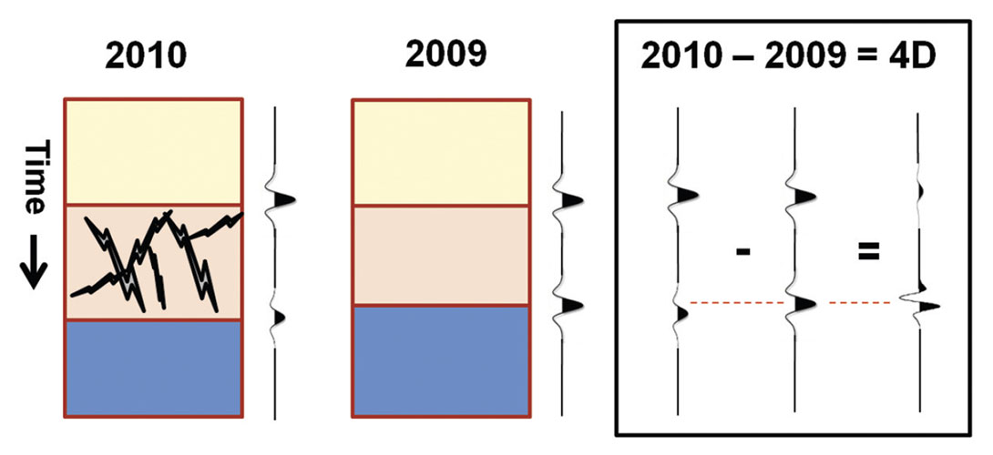
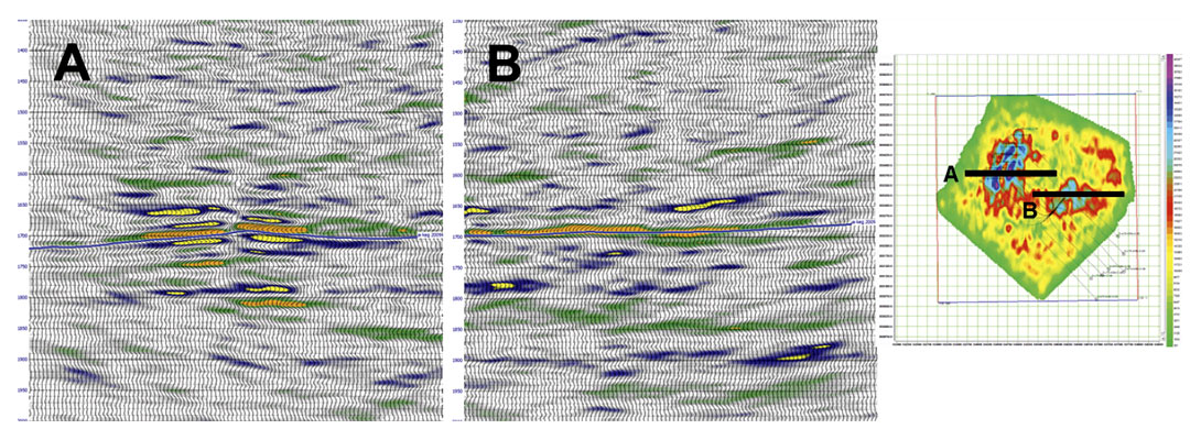
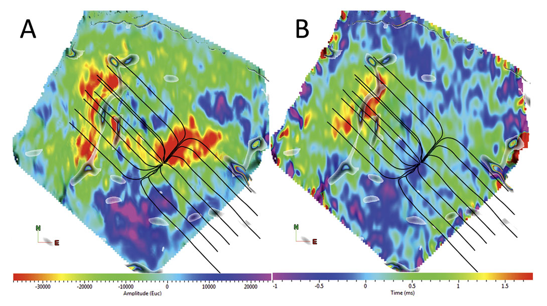
Figure 9 shows the amplitude difference and isochron extracted from the Keg River horizon pre and post frack (2010 – 2009) in an attempt to determine SRV. In the post frack survey, an amplitude decrease on the Keg River is observed predominantly on the west side of the fault. In comparison, there is an increase in traveltime on both east and west sides of the fault with the largest temporal differences occurring east of the fault. An explanation for the observed results is fluid separation in the stimulated zone with gas filled fractures overlying fluid and proppant filled fractures, producing the amplitude and traveltime anomalies on the post stack reflection data. This was hypothesized through an interpretation of a post stack P-impedance inversion on the baseline and monitor surveys (Goodway et al., 2012). This fluid separation could also be occurring spatially with respect to the fault (East/West) but this requires further investigation. The 4D response was concentrated near the toe of the wells for both amplitude and isochron anomalies, and although four wells were completed toe to heel there is no response in close proximity to the heel of the wells. Two possible interpretations are suggested to explain the missing 4D response. First, the gap in microsesimc activity predicts the under stimulated zone and thus there is no 4D response due to lack of stimulation. Secondly, the response is only seen where the refracking of the zone altered the impedances sufficiently to detect a 4D response from hydraulic fracturing. These conflicting results complicate estimating SRV and require further investigation.

Conclusion

The purpose of this investigation was to resolve the EUR variations over the pad by interpretation of the hydraulically stimulated volume through microseismic and 4D responses. It is shown that a gap in stimulation lead to zones of sub-optimal stimulation which reduce EUR over the north pad relative to the south pad. This gap in stimulation, which occurs east of the fault, is thought to be caused by a highly stressed zone. Evidence for the high stress zone causing difficult stimulation is observed in the three independent measurements of high ISIP’s, high closure stress zone in LMR, microseismic gap and low b-values.

Acknowledgements

The authors would like to thank Paul Anderson, Dave Close, David Cho and the Horn River team for their extensive contributions to the project.