Microseismic and Time-lapse Seismic Monitoring of a Heavy Oil Extraction Process at Peace River, Canada

Summary

Peace River is Shell Canada’s in situ heavy oil production operation in northwestern Alberta, with estimated bitumen in place of 7 billion barrels. The current production strategy is to use multi-lateral horizontal wells to steam the bitumen saturated sand reservoir and to then use the same horizontal wells to produce the mobilized bitumen. Although Peace River has been in full-scale operation for almost 20 years, there has been considerable uncertainty about the processes taking place within the reservoir during these steam and production cycles. This has made it difficult to optimize the drilling and operational strategies so as to maximize the value of this large resource. Over the last two years, Shell Canada has carried out a focused effort to apply geophysical monitoring techniques to gain a better understanding of the processes taking place in the reservoir, and to assess the practicality of monitoring on a field-wide basis. Time-lapse surface-to-surface and surface-to-borehole surveys have been carried out, in conjunction with continuous microseismic monitoring, over a number of pads of horizontal wells. The study of this diverse set of monitoring data, together with core and log information, and pressure, injection and temperature data for several steam and production cycles, has provided valuable information about how steam and mobilized bitumen move through the reservoir. This has, in turn, allowed us to adapt our drilling and operational strategy in order to exploit the factors that control steam distribution and ultimately the efficiency of our operation.

Introduction

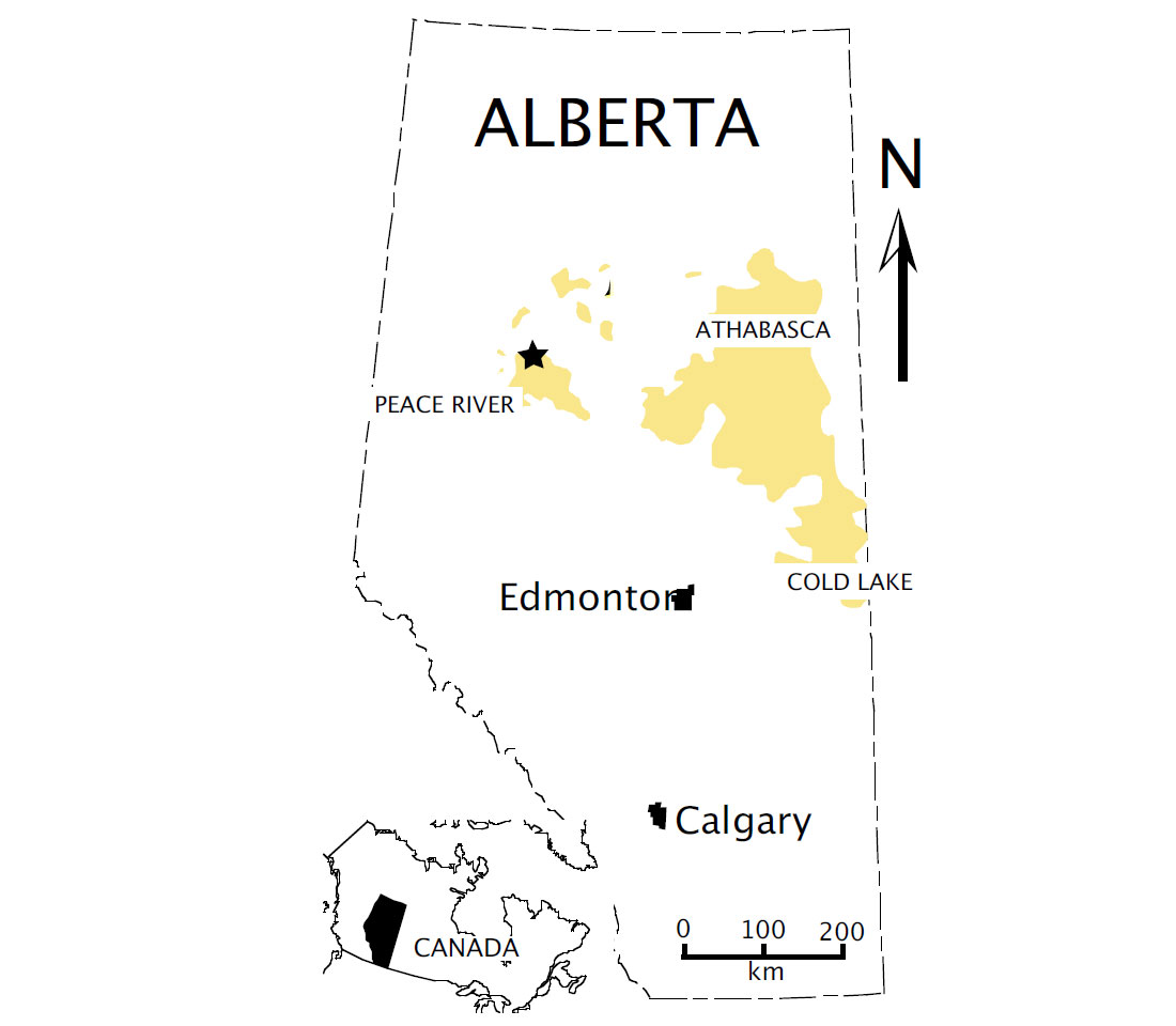
Shell Canada’s Peace River area (Figure 1) consists of several long-term leases totaling approximately 37,000 hectares, with an estimated 7 billion barrels of ~8 API gravity bitumen in place. The exploitable bitumen is found at a depth of about 600 m in sandstones of the Ostracod Zone and Bluesky Formation, which unconformably overlie Mississippian carbonates of the Debolt Formation (Figure 2). In some areas, a non-reservoir Detrital Zone is found at the base of the Ostracod. Reservoir quality is generally excellent, with an average net pay for the area of about 25 m and porosity ranging from 25 to 30%.

Since commercial production began in 1986, several different well designs and techniques have been employed in an effort to extract the bitumen in a cost-effective manner. Grids of vertical injector/ producers, horizontal injector/producers, Steam Assisted Gravity Drainage (SAGD) and Cyclic Steam Stimulation (CSS) have all been tested, with varying degrees of success. The design for the most recently drilled pads of wells makes use of a horizontal well CSS strategy: A series of main boreholes is drilled down to the reservoir from a central pad, and then horizontal laterals are drilled within the reservoir away from the main borehole (Figure 2). Steam is then pumped into the wells at high pressure for several months in order to heat the bitumen and reduce its viscosity to the point where it can flow. Once this has been achieved, the injection of steam is halted and pumps are used to bring the mobile bitumen to surface. After several months, once the flow of bitumen begins to diminish, the steam/production cycle is repeated.

Although the field has been in full-scale operation for almost 20 years, little is actually known about what happens in the subsurface during a steam and production cycle. It has been assumed that the primary mechanism for getting heat into the reservoir is t h rough a combination of dilation and thermal convection outward from the horizontal legs of the wells. This model implies a uniform, cylindrical “steam chamber” that slowly expands on each steam/production cycle. However, it is not known with certainty how steam moves in a lateral sense away from the well bore into the space between well legs or how the steam distributes itself along the length of each of the well legs. There is also uncertainty in terms of how the steam distributes itself vertically in the reservoir. Given the uncertainties associated with the entire steam/ production process, it would seem important to better understand what is happening within the reservoir in the hopes of controlling and then optimizing the operation. An experiment incorporating multiple remote sensing techniques and applied to the CSS process over a single test pad of wells was thus proposed as a way of gaining a better understanding of reservoir processes and of evaluating the use of these technologies for field-wide monitoring.

Experiment

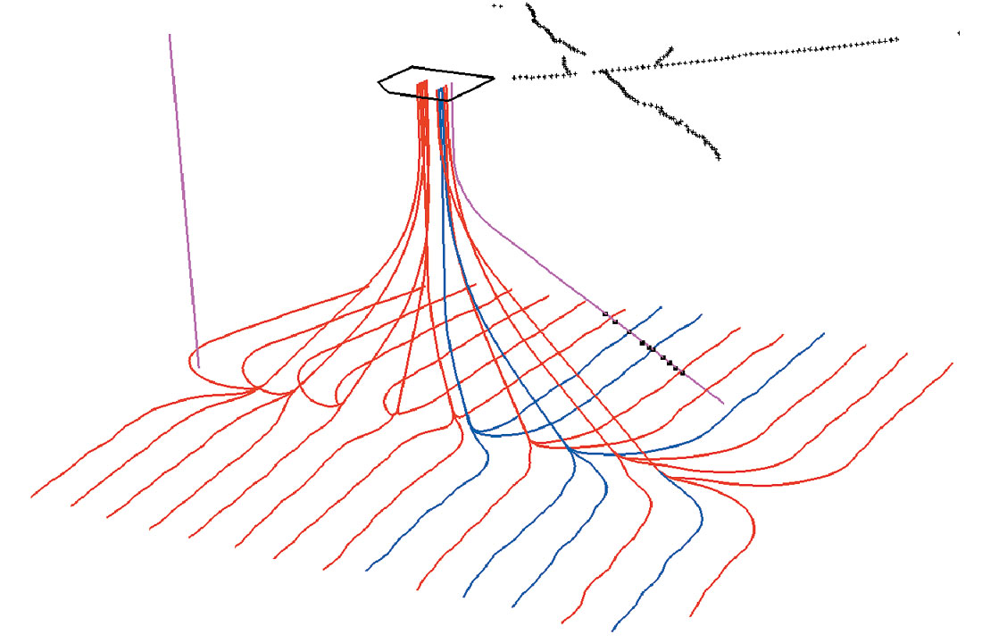
The monitoring experiment focused primarily on the application of time-lapse seismic and microseismic monitoring. In addition, surface tiltmeter monitoring was also evaluated, but will be discussed in a future paper. Pad 40, a pad of horizontal CSS wells (Figure 3), was selected for the experiment and a 50 level array of 3 component geophones was cemented into place in the deviated observation well TH40-A. A cross-spread of permanent source locations was created by drilling and casing 15 m deep shot holes along two orthogonal lines above the observation well. The geometry of the geophone array and shot locations is shown in perspective view in Figure 3. For a particular survey, each shot was fired off and the resulting reflection seismic record was recorded at each of the 50 subsurface geophones, as well as at surface geophones located at each of the shot locations. This unique acquisition geometry yielded a 3D VSP, as well as a pair of high-fold 2D seismic lines and a very sparse (one fold) surface 3D. In addition, when the active surveys were not being carried out, the array could be used to passively “listen” for microseismic events associated with fracturing caused by the movement of steam within the reservoir.

The deployment of the VSP/microseismic array took place in September 2002 – several weeks prior to when first steam was to be injected into the pad. A baseline 3D VSP and surface-to-surface seismic survey were carried out, and the microseismic recording began. Three repeats of the 3D VSP and surface-to-surface seismic survey have since been carried out at the end of each of two steam cycles, and a repeat at the end of a production cycle has also been acquired.

Results of the Experiment

It was hoped that the combination of microseismic and time-lapse data sets could be used to infer the location of the steam front and help us understand the mechanism through which the reservoir is heated. Figure 4 shows the locations of microseismic events recorded over the course of the first steam cycle. Clearly, the large number of events indicates that fracturing of the reservoir is indeed taking place – suggesting that our original model for the process of getting steam into the reservoir is incorrect. As well, the fracturing is not uniformly distributed, with some areas experiencing extensive fracturing, while others being relatively inactive. This suggests that our assumption of uniform steam distribution and good steam conformance is also not correct. Finally, NW/SE trends in the microseismic event locations suggest that fracturing within the reservoir will follow corridors of weakness that appear to be influenced by regional and in some cases more localized, deep-seated structures.

Although we were confident that the VSP part of the time-lapse effort would yield detailed information over a small region below the observation well, problems with a strong reflected shear wave event that is superimposed on the zone of interest have so far hampered our efforts to process and interpret the data. Fortunately both the high-fold 2D lines and the sparse 3D that were acquired with the VSP responded well to conventional time-lapse processing.

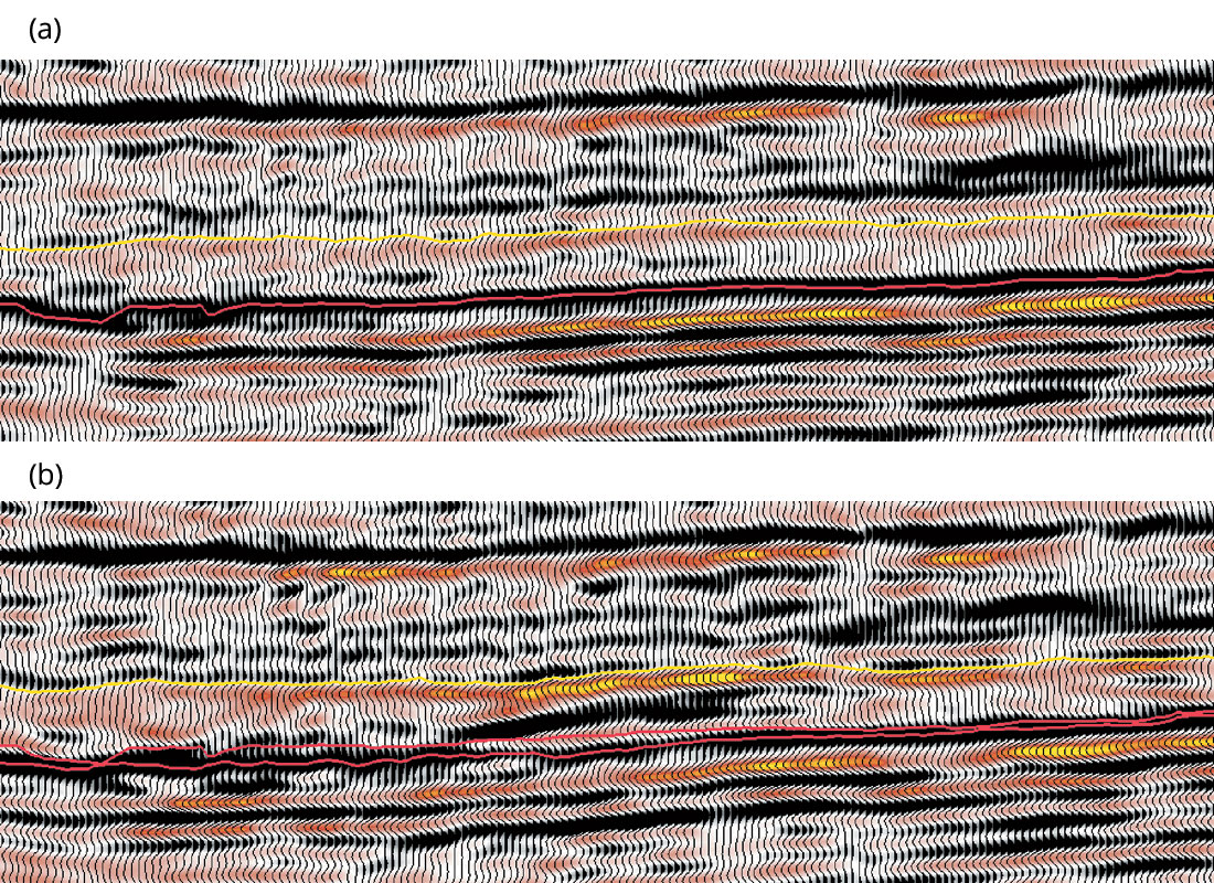
As can be seen in a comparison of the baseline and first repeat seismic sections for the NE/SW high-fold 2D line shown in Figure 5, large time-lapse effects were observed at the reservoir level as a result of heating of the bitumen. Interestingly enough, the bulk of the heating was seen to be taking place at the top of the reservoir – well above the horizontal legs of the injectors that had been drilled along the base of the reservoir.

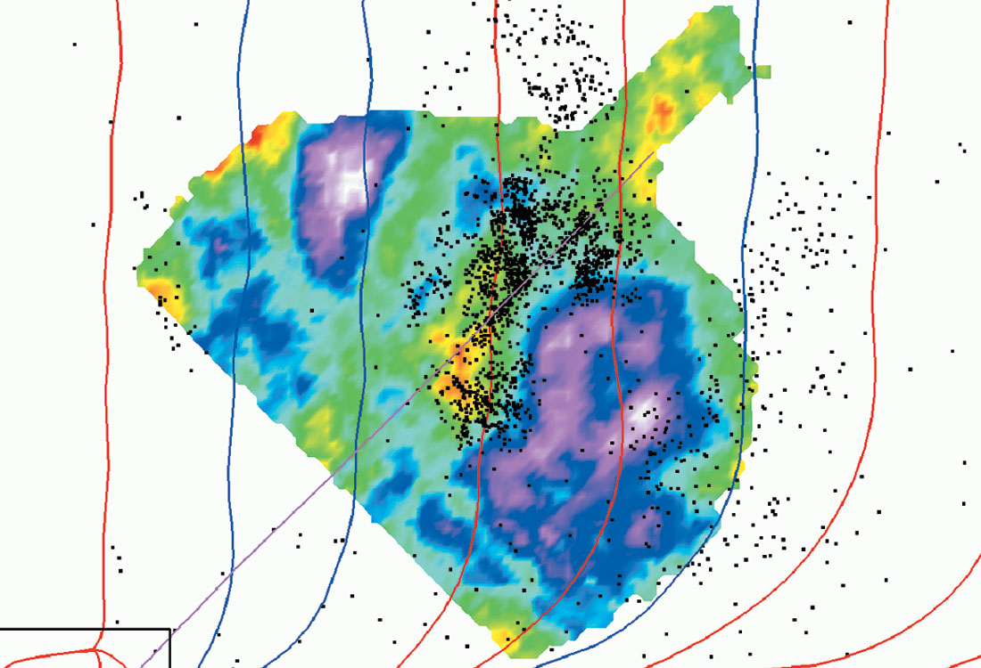
In spite of its sparseness, the low-fold 3D that was acquired as part of the time-lapse acquisition proved to be of surprisingly good quality and showed similar time-lapse anomalies. A map of the amplitude of these anomalies (Figure 6) shows areas where heating has been concentrated, and areas where steam appears to have not yet reached. Given what we know from core about the distribution of more permeable sands below the pad, it appears that more extensive heating is taking place in the areas where these better quality, more permeable sands are located, and that steam is avoiding those areas that are less permeable. Comparing the microseismic event locations to the time-lapse data (Figure 6) revealed that microseismic energy is concentrated along the edge of the heated zone, where steam would be fracturing the rock as it encounters less permeable reservoir. Continued monitoring of microseismic data through the course of two more steam cycles and further repeats of the time-lapse survey indicated that the heated zone had grown somewhat, expanding into the area where earlier fracturing had occurred.

Towards Field-wide Monitoring

Building on the efforts of the Pad 40 experiment, microseismic installations have now been deployed at two more production pads. A fourth array is currently being deployed and will be used to monitor a new pad of wells, and two additional deployments are planned for the new year.

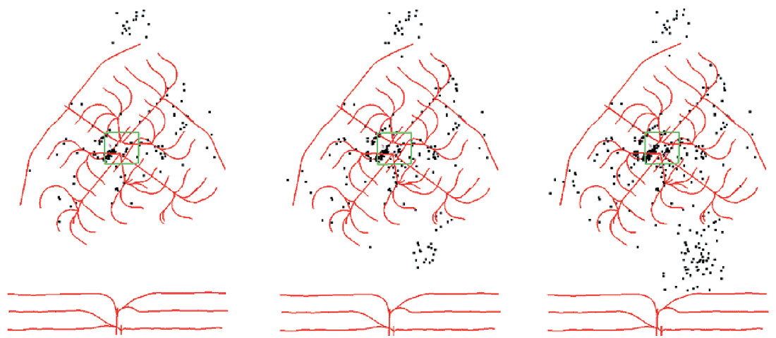
Results from the new installations have continued to provide valuable information about our operations. For example, microseismic monitoring at Pad 30 over a full steam cycle revealed a relatively homogeneous fracture distribution up until the point where the pressure at Pad 30 reached its maximum and the pressure at Pad 31, its sister pad on production to the south, reached its minimum. The sequence of images in Figure 7 reveal a large fracture or fracture network that moved quickly across the buffer zone between the two pads. No doubt the large pressure gradient resulted in extensive fracturing in the reservoir across the buffer zone and established fluid communication between the two pads. This was confirmed by examining pressure and production/injection data from the wells closest to the buffer zone. Fortunately, steam injection at Pad 30 was terminated just as the swarm of microseismic events reached Pad 31, avoiding the possibility of steam breakthrough into the producing wells.

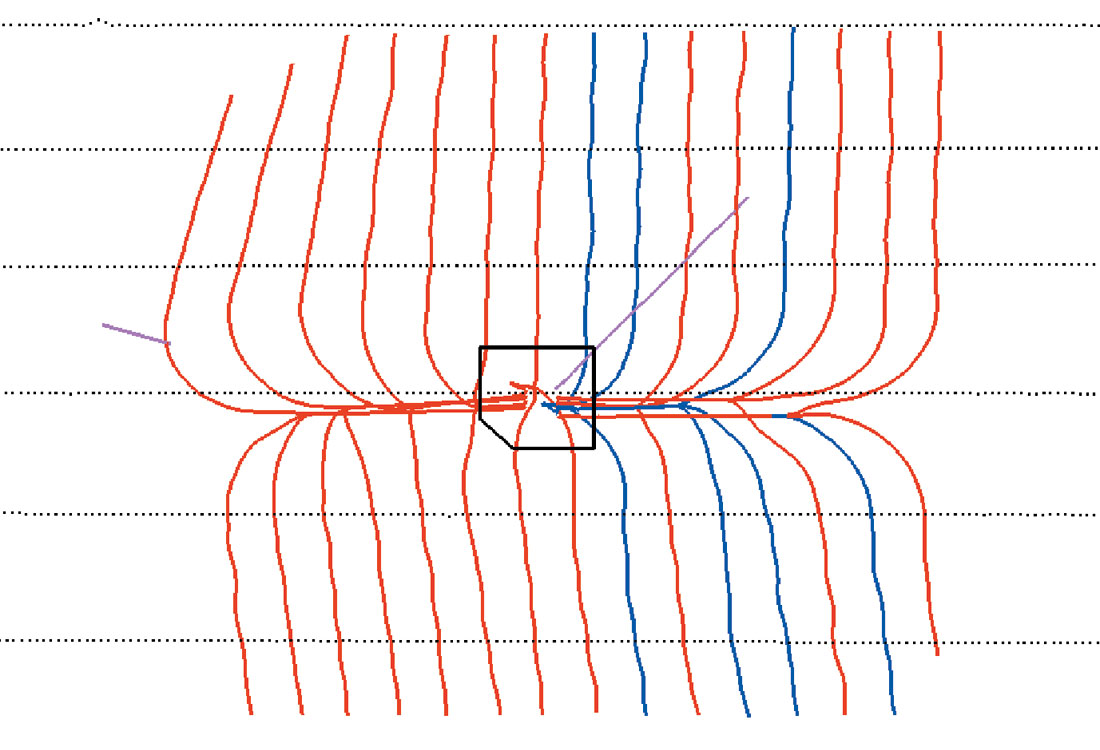
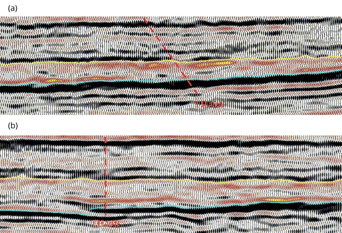
In addition to the new microseismic installations, we are also carrying out more extensive time-lapse seismic programs over entire pads. Figure 8 shows the shot points for a 2D swath program that was repeated this spring over Pad 40. Two seismic sections from the swath repeat that traverse wells with thermocouples installed across the reservoir interval are shown in Figure 9. In Figure 9a, the section ties TH40-A, where no increase in temperature has been observed over the entire reservoir interval even after three full steam cycles. High temperatures, however, are indicated on the seismic section on either side of the thermocouple string at the top of the reservoir. In Figure 9b, the section ties TH40-B, where a large increase in temperature has been observed from the thermocouples over the lower 5 m of reservoir – the upper 20 m of reservoir is essentially cold. Note that the temperature anomaly on the seismic section at the well tie indicates heat in the bottom part of the reservoir and no heat in the upper part and is consistent with what the thermocouple data have shown. These ties of the time-lapse seismic to the thermocouple data at two wells gives us excellent calibration information. We see, for example, that the pressure effect on the seismic at the end of a steam cycle is uniform across the reservoir and leads to about a 17% decrease in the P-wave velocity. The temperature effect that we see at TH40-B leads to an additional 21% decrease, but is of course more localized.

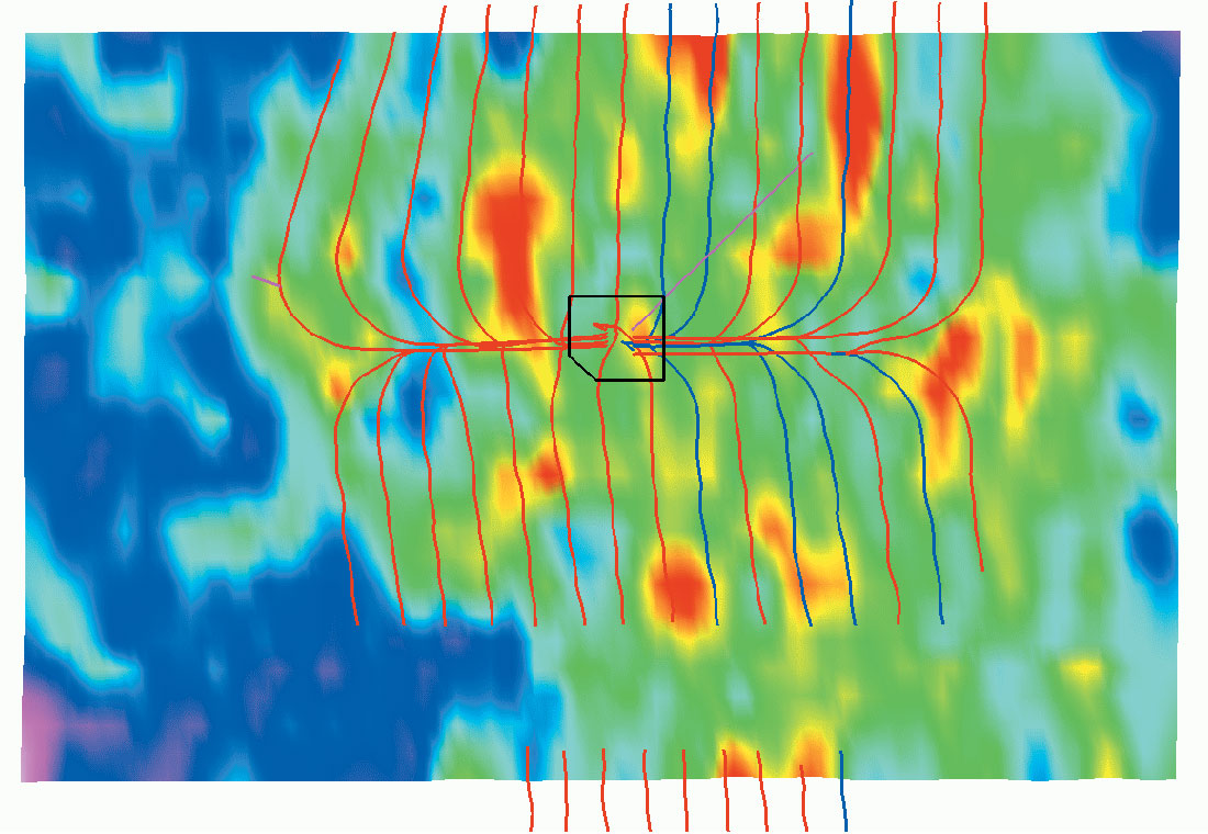
To highlight the areas where steam has been successful in heating the bitumen, the maximum negative amplitude of the swath seismic data over the reservoir interval provides a simple but effective attribute. A map of this attribute for Pad 40 after three steam cycles is shown in Figure 10. Note that the distribution of heat, as indicated by reds and yellows on the attribute map, is quite non-uniform. In general, only one of the three laterals that kick off from each of the main boreholes is seen to be putting significant steam into the reservoir – indicating that the use of multi-lateral wells is hurting steam conformance. There is also a strong correlation between the trajectories of the laterals through specific intervals in the reservoir and the preference for steam to move into the reservoir. Where laterals encounter more permeable, coarser grained reservoir sand, or when they traverse zones that are under higher stress conditions due to deeper structures, these zones act as conduits for the steam and the result is the patchy heat distribution seen in Figure 10. Clearly taking the local geology into account prior to designing the well trajectories could be key to enhancing the productivity of the wells.

Conclusions

From the results of this work it was concluded that the initial model of a uniform, conductive heating process was incorrect, and that steam distribution is in fact quite non-uniform, with some areas of the reservoir receiving the bulk of the steam, and other areas receiving very little. Steam distribution, in fact, appears to be strongly influenced by geology, with higher permeability zones acting as conduits for steam when they are encountered. The generation of fracture networks within the reservoir also appears to be an important mechanism for getting steam into the less permeable regions of the reservoir. Deep-seated structures that create stressed zones in the reservoir appear to control the development of these fractures. Clearly, the influence of geology and the regional and local stress pattern within the reservoir must be considered when designing, drilling and operating development wells. As well, knowing now that fracturing is an important mechanism for pushing steam into less permeable parts of the reservoir, the need for controlling pressures and pressure gradients becomes evident. Microseismic monitoring can be used, in fact, as a tool for determining on a well-by-well basis how successful we have been in creating new fractures for a given steam cycle. It also allows us to monitor the caprock integrity and the interaction between injectors and producers to prevent steam breakthrough.

Acknowledgements

The author would like to thank Ted Urbancic and Shawn Maxwell for the work that Engineering Seismology Group (ESG) has carried out on the microseismic part of this project. As well, thanks are due to Robert Pike and Rod Couzens of Sensor Geophysical for their time-lapse processing and analysis. Thanks also to Rodney Calvert, Matthias Hartung, Jim Clippard, Karel Maron, Stephen Bourne, Dan Pribnow, Krijn Witt, Charles Jones, Andrey Bakulin and Steve Oates from Shell Exploration and Production Technology and Research (SEPTAR) for their technical support in the early stages of the project, and their contribution to our understanding of the different data sets and the development of a conceptual reservoir model for Peace River.