Multivariate Geostatistics

1.0 Introduction

Multivariate geostatistics is a broad term that encompasses all geostatistical methods that utilize more than one variable to predict some physical property of the earth. Bivariate geostatistics is obviously the simplest subset of the multivariate techniques and thus the standard technique of cokriging could be called multivariate geostatistics. However, in this paper we will use the name to refer to geostatistical methods that use more than two variables. Even then, there are many different methods that fall under this heading. There are three major subcategories:

1. Methods that produce an output value from a linearly weighted sum of the input values.
2. Methods that use artificial neural networks (ANN's) to combine attributes.
3. Methods which construct a final answer using principal component analysis.

In this paper, we will be considering only techniques described in point (1). For a discussion of point (2), refer to a series of papers in The Leading Edge by Ronen et al (1994). For a discussion of methods in point (3), refer to the textbook by Wackemagel (1995).

2.0 Using Seismic Attributes to Estimate Log Properties

The idea of using multiple seismic attributes to predict log properties was first proposed by Schultz et al (1994), in a series of TLE articles. In these articles they point out that the traditional approach in using seismic data to derive reservoir parameters has been to look for a physical relationship between the parameter to be mapped and some attribute of the seismic data, and then use that single attribute over a 2D line or 3-D volume to predict the reservoir parameter. Examples of such attributes include:

1. Analysis of the seismic trace itself for amplitude increases, which indicate changes in reflection coefficient size, since; for example, if the acoustic impedance shows dramatic changes, as in a gas sand, so should the seismic trace.
2. Extraction of the acoustic impedance from the seismic data by integration. Of course, the result will lack a low frequency component due to the effect of the seismic wavelet. This is often corrected for by adding the low frequency component from a well log model. (Schultz et al object to calling the result a seismic attribute, since it has already been influenced by the well log data).
3. The use of prestack data to extract information about intercept and gradient, and hence Poisson's ratio or shear wave reflectivity.
4. The use of instantaneous attributes derived from the seismic data. These attributes are based on the definition of the complex trace, which, in polar form, give us the three classical seismic attributes: the amplitude envelope, instantaneous phase, and instantaneous frequency. These are the three primary attributes, but many more can be derived from the basic three.
5. New attributes which have been introduced recent!y, such as coherency. Indeed, any seismically derived attribute can be introduced into this discussion.

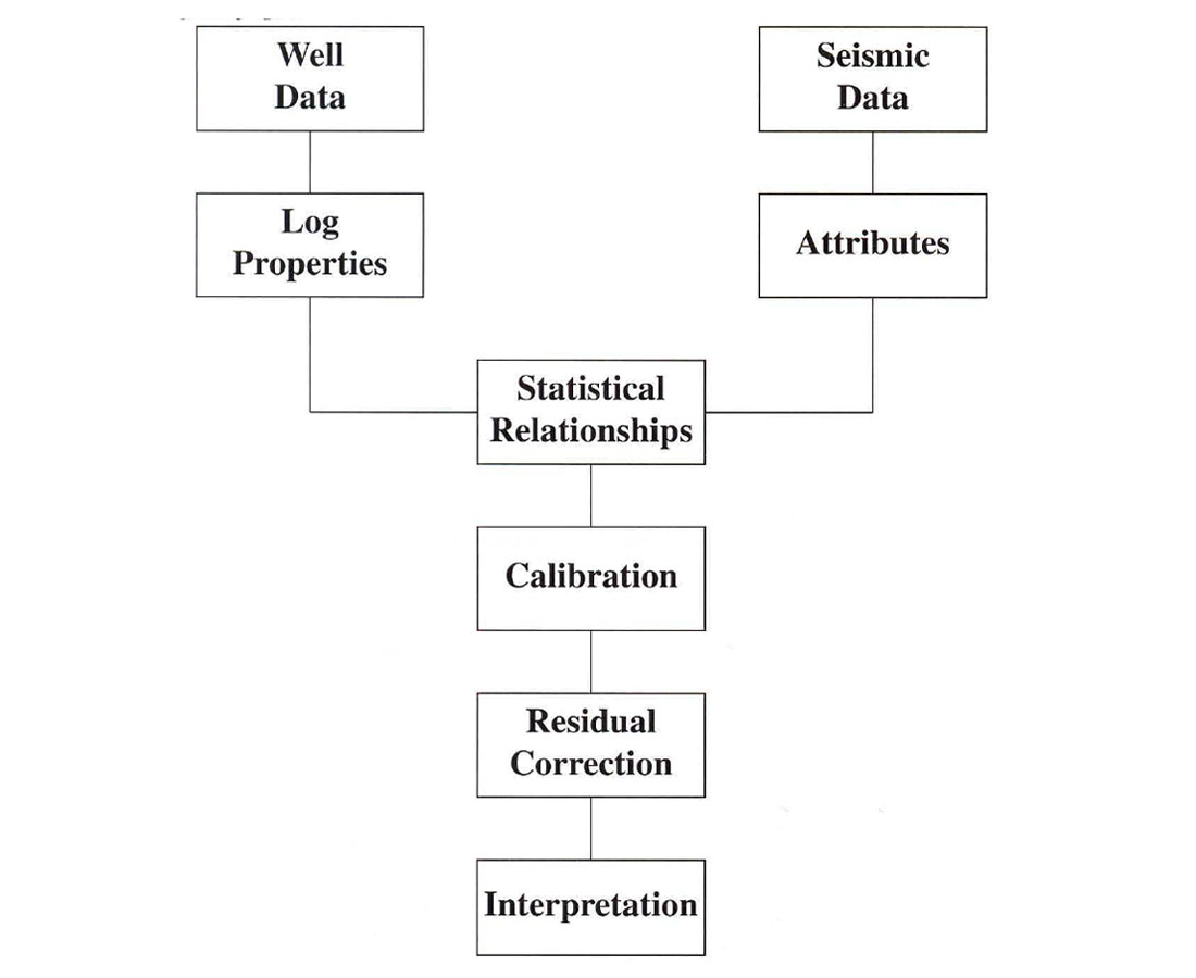
Although relationships have been inferred between these attributes and reservoir parameters, the physical basis is not always clear, and we may want to derive statistical, rather than deterministic relationships. This approach, which Schultz et al call a data-driven methodology, is summarized in Figure 1.

In the most general case, we look for a function that will convert m different attributes into the desired property. This may be written:

P(x,y,z) = F[A₁(x,y,z,), .... , A_m(x,y,z)] (1)

where:

P = The property as a function of coordinates x, y and z.

F = The functional relationship,

A_i, i= 1, ... , m = the m attributes.

The simplest possible case would be a linearly weighted sum:

P = w_o+W₁A₁+ ....w_mA_m (2)

Obviously, this raises two questions: which attributes should we use, and how do we judge their quality. The number and types of attributes must be determined geophysically, and the quality of the attributes can be determined using crossplots between the attributes and the parameter to be measured.

As an example of such a linear function, let us consider:

ϕ(x,y) =W₀+ w₁I(x,y) + w₂E(x,y) + w₃F(x,y) (3)

ϕ(x,y) = Porosity
I(x,y) = Acoustic impedance,
E(x,y) = Amplitude Envelope,
F(x,y) = Instantaneous frequency, and
     w_i = weights

In the above example, the reservoir zone is given by the vertical average of a spatially varying time zone over a picked seismic surface. The question now becomes how we determine the weights w_i . One approach would be to first calculate an estimate from the well logs using kriging. The problem here is that you need a fairly large number of well logs in the area to come up with a reliable map estimate. A second approach would be to estimate the coefficient over longer depth or time zones calculated at the well logs themselves:

ϕ(t) = W₀+ w₁I(t) + w₂E(t) + w₃F(t) (4)

where:

ϕ(t) = porosity at the well integrated to time and calibrated to the seismic data.

For both of equations (3) and (4), the solution can be arrived by using the least squares approach.

The attributes used in the linear sum can then be measured for goodness of fit with the parameter to be predicted by use of the correlation coefficient between each variable, given by:

where:

σ_AP = covariance between A and P,
σ_A = standard deviation of A,
σ_P = standard deviation of P,
A is the attribute, and
P is the parameter.

If we have N attributes, there will be N!/(2!(N-2)!) correlation coefficients, and these can be ordered from best to worst. However, it should be noted that when we determine the best combination of attributes to use in the final sum, the order of the attributes used may not be the same as the order of their correlation coefficients. This may seem strange at first, but consider a simple example. One of the attributes could just be a linearly scaled version of another attribute, and it would obviously have just as good a correlation coefficient. But adding this attribute to the sum would not improve the fit.

The quality of the fit can be determined by finding the RMS error between the known parameter and the estimated parameter. By using this criterion, we can find the optimal combination of attributes to use.

An example of the preceding equations applied to estimates of porosity between a well log and a seismic section will now be shown.

3.0 A Case Study Using the Weighted Sum Method

As an example of the technique described in the previous section, we will look at a case study involving the prediction of sonic logs at various locations along a seismic line from Alberta. The attributes used were as described in the previous section:

Bandlimited acoustic impedance, found by integrating the trace. The reflection coefficients were the trace samples themselves normalized by dividing by the maximum absolute amplitude on the trace and multiplying by 0.25.

Amplitude envelope of the seismic trace. Instantaneous frequency of the seismic trace.

The seismic time itself, used as a ramp function to introduce the DC bias and low frequency content.

Note that the porosity was actually derived from a set of sonic logs using Wyllie's equation:

ϕ = (Δt - Δt_ma)/(Δt_f - Δt_ma), (6)

where:

Δt = sonic transit-time,
Δt_ma = matrix transit-time, and
Δt_f = fluid transit-time.

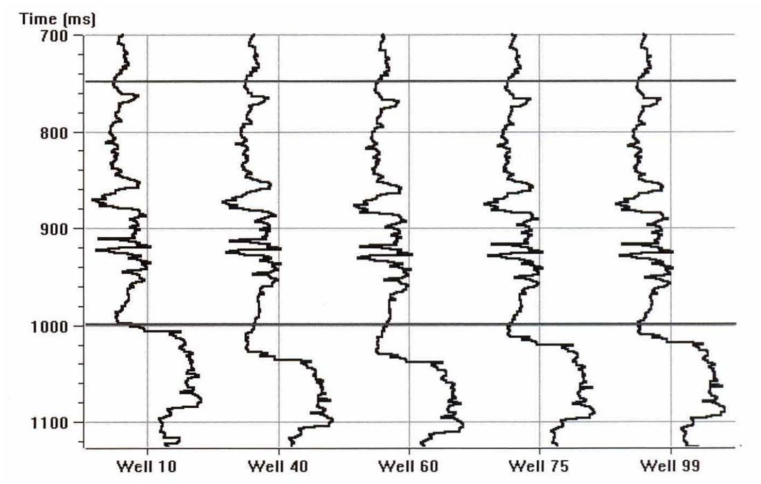
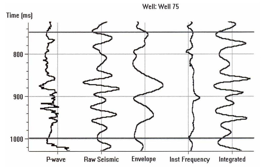
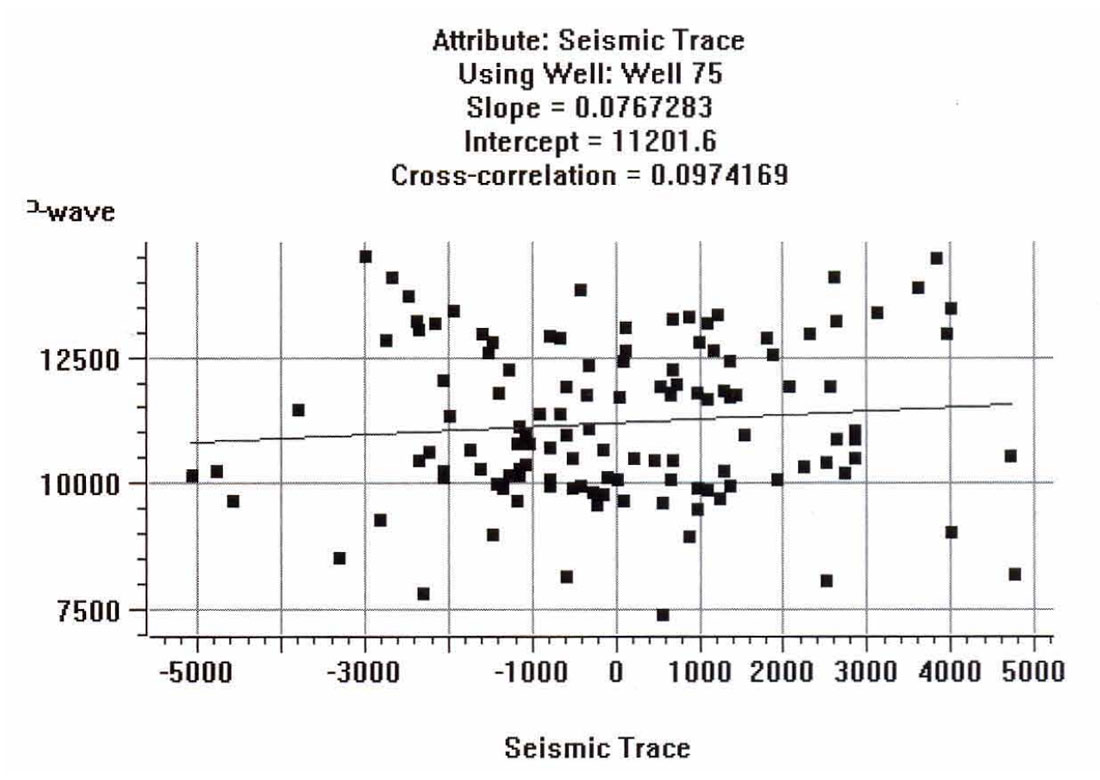
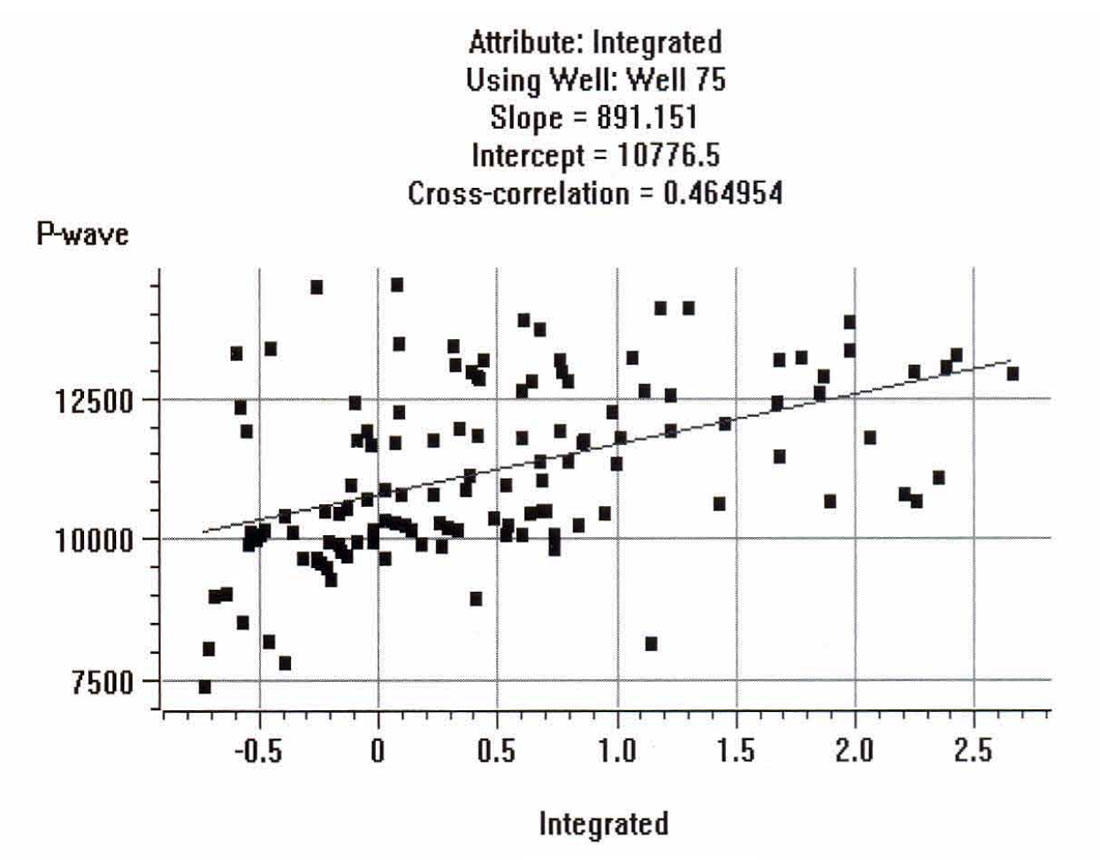
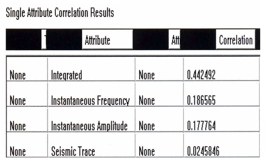
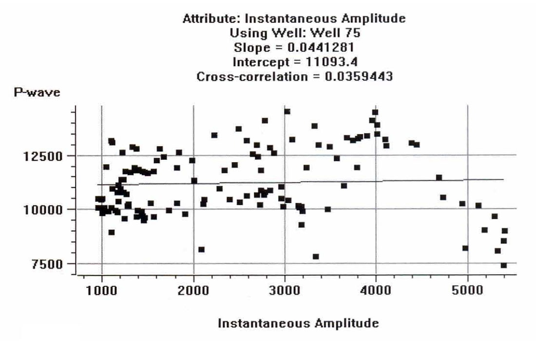
The sonic logs are shown in Figure 2. Only one of them, well 75, is actually a measured sonic log. The others were derived from well 75 by stretching and squeezing the log so that the derived synthetics matched the seismic trace from the same location. The bars on the plot show the zone of interest, which covers a series of Cretaceous events, but does not extend into the higher velocity Devonian events. Figure 3 shows the attributes calculated for well 75, where we have included a display of the seismic trace. The reason that it was felt that the integrated trace should be used rather than the original trace is found when we crossplot the attributes against the P-wave sonic. Figures 4 through 7 show the crossplots of the seismic trace, integrated trace, amplitude envelope, and well 75 sonic. Notice that the seismic trace displays the poorest correlation when correlated against the sonic log values. When all 5 wells are taken into account, the situation is magnified even more. Table 1 shows the averaged correlations of all 5 wells, with the seismic trace by far the worst.

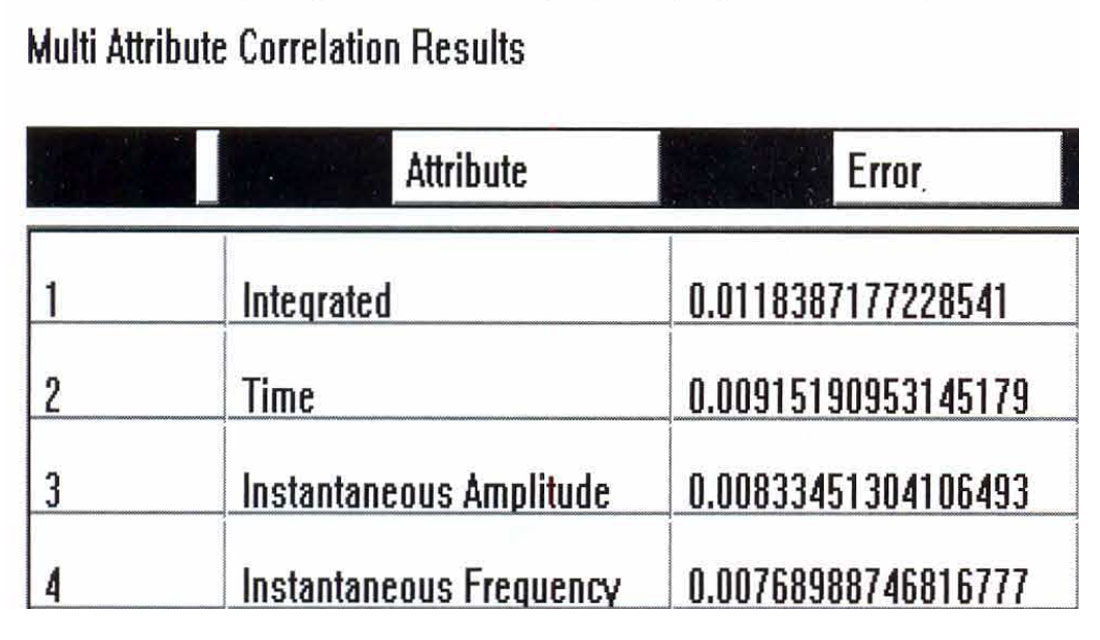
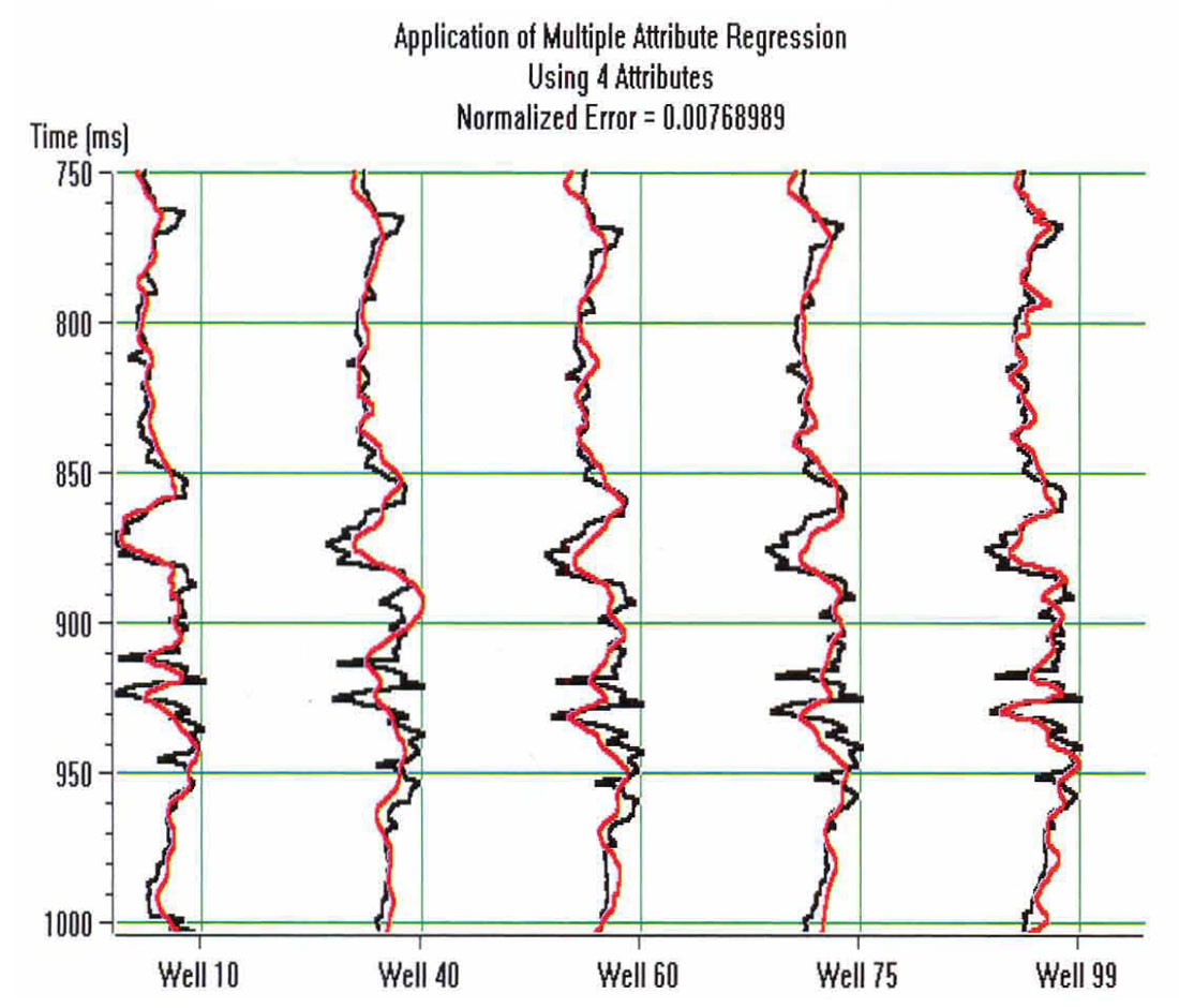
Next, the multi-attribute analysis was done, using a 30 point, symmetrical operator. Table 2 displays the numerical results, showing the residual error after the addition of each attribute. Figure 8 shows the final result, with the predicted trace superimposed on the original trace.

Conclusions

In this paper, we have shown a fairly straightforward example of the use of multivariate geostatistics. We have concentrated on the prediction of a well log parameter using a weighted sum of seismic attributes. The result, shown in Figure 8, is surprisingly good when you consider that no geological information was used to predict the sonic logs. That is, they were recreated simply by a linear convolutional sum of three seismically derived attributes. The linear operators were created by "training" the program using the techniques of geostatistics. This simple example was just to demonstrate the concept. By using more attributes (with the caution that there is an optimum number that should not be exceeded) and other techniques (such as Artificial Neural Networks), the prediction can get even closer.

Obviously, there are many other applications of the technique that we have just shown. It is our feeling that the introduction of geostatistical techniques to our industry gives us a powerful tool which will challenge the deterministic model of seismic processing and lithology prediction that has been in use for so many years.