On the extraction of angle dependent wavelets from synthetic shear wave sonic logs

Summary

The extraction of angle dependent wavelets requires the use of a shear wave sonic log. However, shear wave measurements are often not acquired in a conventional logging suite and must be estimated to produce a synthetic result. The errors associated with the synthetic shear propagate through to the angle dependent reflectivity with a sine squared dependence of the incidence angle. Therefore, the reflectivity becomes unreliable at larger angles and a least squares extraction using the convolutional model could yield erroneous results. To reduce the errors associated with wavelet extraction at larger angles, a near angle wavelet was estimated with an acceptable amount of error using a least squares approach. Subsequently, an estimate of the angle dependent wavelet amplitude spectrum and a constant Q attenuation model was used to evolve the amplitude and phase respectively to estimate the wavelets at larger angles.

Introduction

In an amplitude variation with offset (AVO) inversion, the seismic wavelet is used in the forward modeling process where it is convolved with a model reflectivity to generate the synthetic seismic data. Due to the attenuation effects of the Earth, the wavelet is non-stationary and alterations in the amplitude and phase occur throughout its propagation history. Therefore, in an AVO inversion where multiple angle dependent measurements of the reflection response are used, separate wavelets for each angle can be used to compensate for the attenuation effects as a result of increased propagation distance with larger angles.

The extraction of the wavelet is typically performed using the concept of the convolutional model, which states that the seismogram is the result of a convolution between a reflectivity series and a wavelet. Using this method, a reflectivity series must be generated and is typically performed using well log measurements and an appropriate formulation of the angle dependent reflectivity. The required well logs then consist of the compressional and shear wave velocity and the density. The compressional wave velocity and density logs are typically included in a standard logging suite. However, the shear wave velocity is often not acquired. In such cases, statistical methods can be used for wavelet estimation but will lack the associated phase information. An alternative option is to generate a synthetic shear wave sonic log using an appropriate method. However, finite errors will exist in the synthetic shear and will subsequently propagate through the wavelet extraction process, degrading the final result. This study investigates the errors associated with wavelet extraction using a synthetic shear wave sonic log and proposes the use of a constant Q model to evolve the wavelet for reducing the errors associated with the final extracted wavelets.

Synthetic shear generation

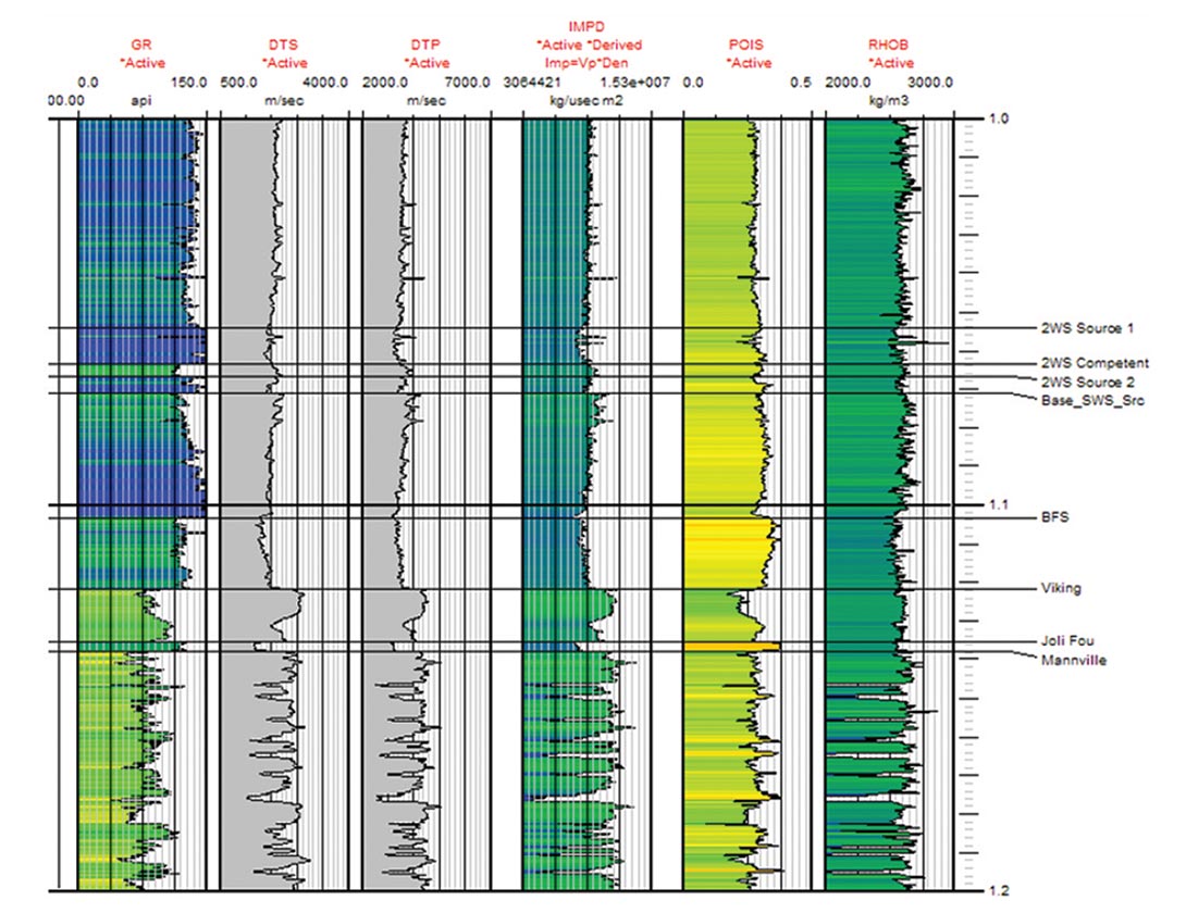
Numerous methodologies exist for estimating the shear wave velocities including the use of rock physics models or making simple assumptions such as a constant compressional to shear wave velocity ratio. Here we implement a methodology using a linear transform between the compressional and shear wave velocities derived from nearby wells with measured shear wave information. The well used to derive the transform relationships are first separated into distinct lithologies using various well log measurements as illustrated in Figure 1.

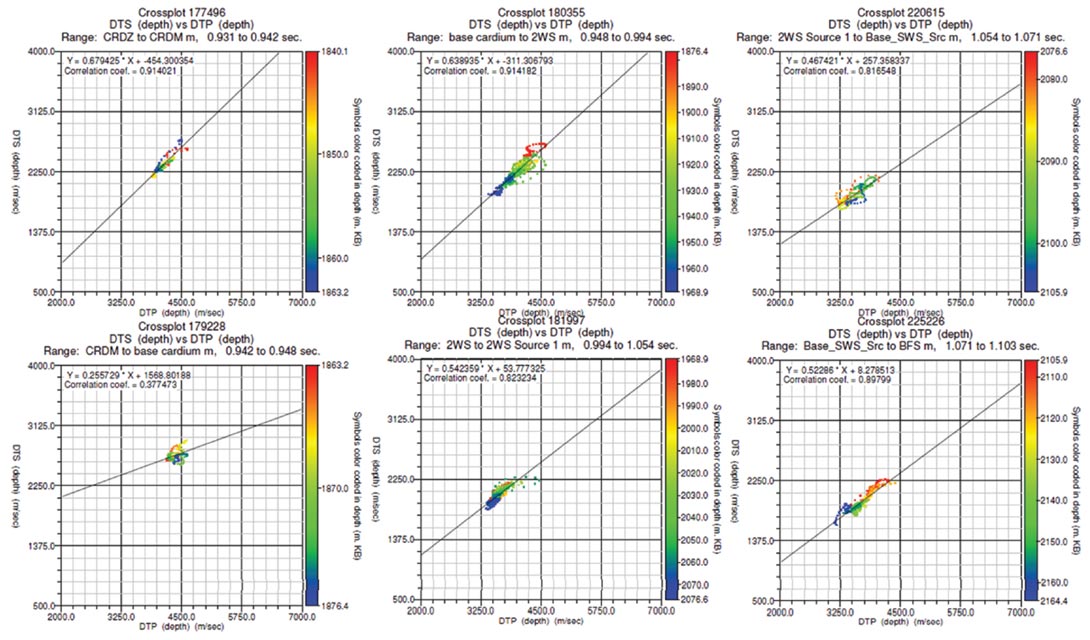
Subsequently, a linear regression is performed for each defined lithology using a scatter plot of the compressional and shear wave velocity values. Figure 2 shows the regression analysis for the defined lithologies in Figure 1. These relationships are then applied to the compressional wave velocities at the estimation well to generate the synthetic shear.

The derived regression line forms a linear transform relationship between the compressional and shear wave velocities for each defined lithology that is analogous to the mudrock line of Castagna et al. (1985). A measure of the associated errors can be obtained by the scatter of points around the mudrock line and will have a value that is on the order of the standard deviation for the associated distribution. Typically, data points for shales (mudrocks) and clean sands will fall along the mudrock line, whereas tight gas sands will deviate from this trend (Castagna et al., 1985) as can be seen in Figure 2. Therefore, the analysis is more ideal for shale formations and clean sandstones.

Wavelet estimation errors

For the extraction of the angle dependent wavelets from measured well logs, we use the convolutional model, which is given by

where s is the seismogram, w is the wavelet and R is the reflectivity convolutional operator. The single and double underlines represent vector and matrix quantities respectively. In addition, each quantity is dependent on the incidence angle, θ. The resulting least squares solution for the wavelet is given by

To solve equation 2, we must calculate the angle dependent reflectivity from the well logs and construct the corresponding reflectivity convolutional operator. Consider a simple two term AVO equation given by

where r is the reflectivity and A and B represent the compressional and shear wave velocity terms respectively. Differentiation of equation 3 with respect to the shear wave velocity term yields

Equation 4 states that for a given error in the shear wave velocity, the corresponding error in the reflectivity as a function of θ has a sine squared dependence. This is illustrated in Figure 3.

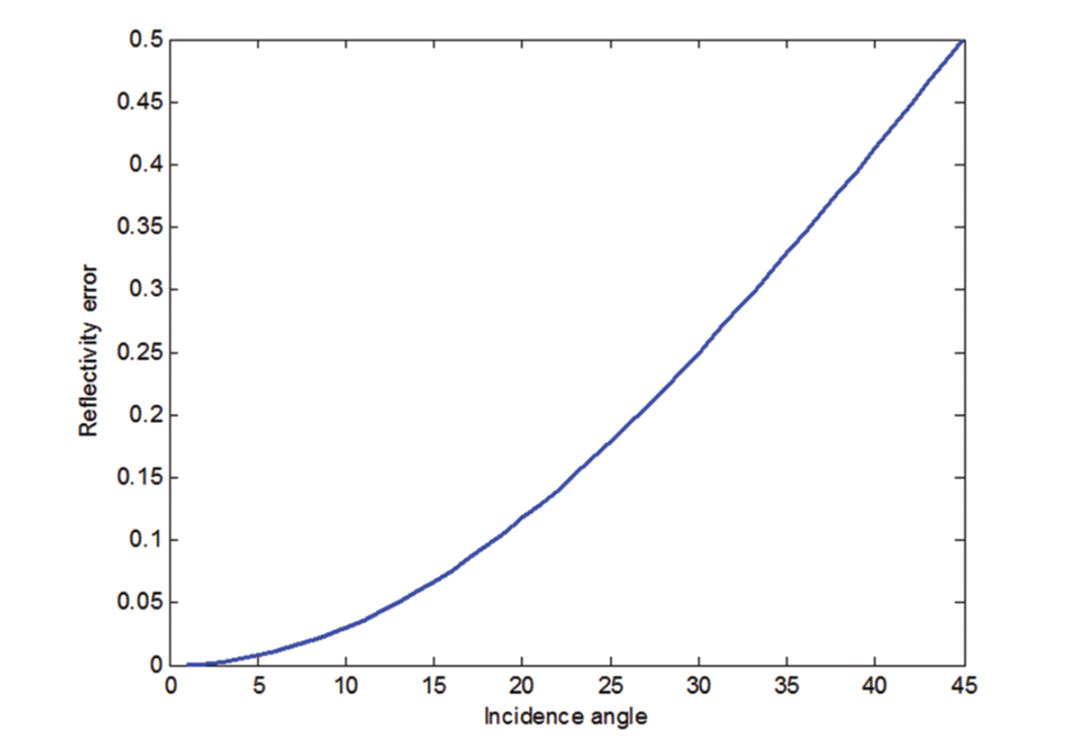
The error in the reflectivity is low at near angles and increases for far angles. Therefore, at far angles where significant errors are present, the seismogram will fall outside the column space or range of the corresponding reflectivity convolutional operator. Consequently, the angle dependent wavelets extracted using equation 2 will be increasingly unreliable with increasing angle. Using the least squares extraction method, the only wavelets that can be relied upon are the near angle wavelets that contain a relatively small amount of error.

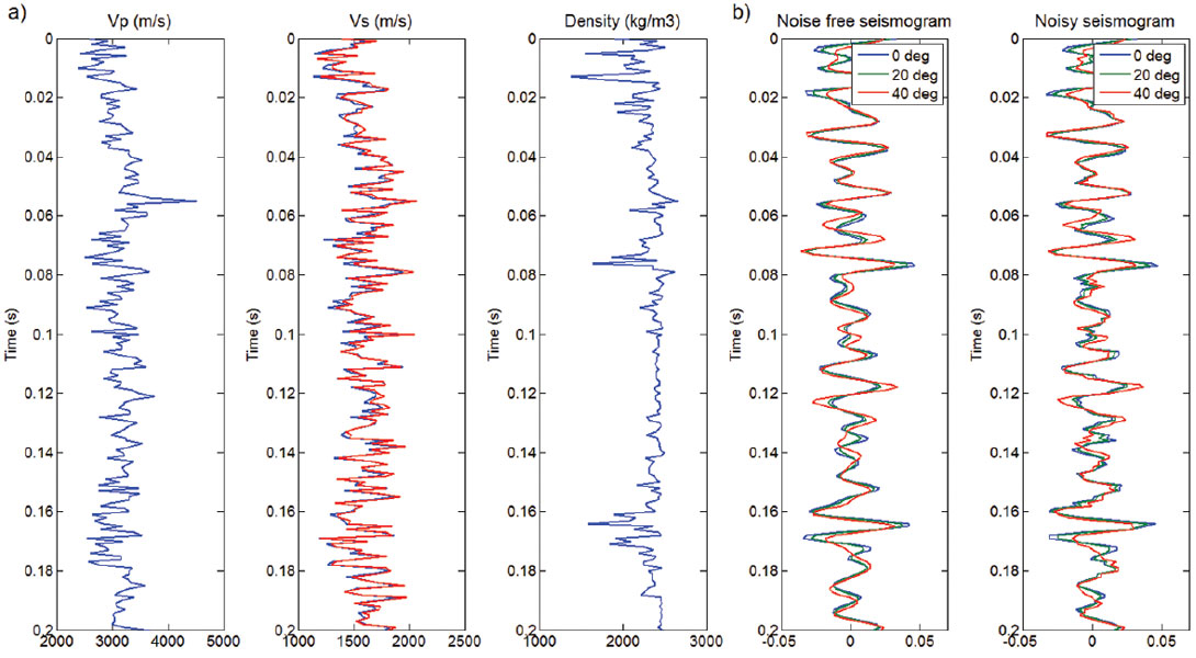
To illustrate the effects of a least squares wavelet extraction when shear wave velocity errors are present, we consider a synthetic example. Figure 4a shows the compressional and shear wave velocity and density logs used in the analysis. The curves shown in blue represent the error free logs and the red curve represents the shear wave velocity log with finite errors. The errors were generated through the addition of uniformly distributed random noise with a maximum error of 10 percent. Using the blue curves and the Aki and Richards (1980) approximate AVO equation, we generate the angle dependent reflectivity for zero, 20 and 40 degrees angle of incidence. The corresponding seismograms upon convolution with a Ricker wavelet are shown in Figure 4b where a noise free and a noisy case are considered. Again, the noisy seismograms were generated through the addition of uniformly distributed random noise with a maximum error of 10 percent. These are the seismograms from which the wavelets were extracted.

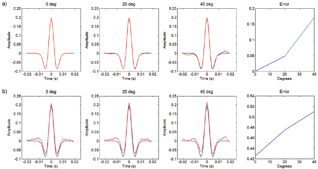
For the extraction of the wavelets, we generate the reflectivity convolutional operator using the red shear wave velocity log shown in Figure 4a and solve the corresponding system of equations given by equation 2. Figure 5 shows the extracted wavelets for each angle with and without the addition of noise. In addition, the sum of the absolute value of the difference between each extracted wavelet and the original wavelet is shown. Note that for the noise free case, the associated error is zero for an angle of zero and increases with an increasing angle of incidence. For the noisy case, the errors are substantially greater for a minimal amount of added noise. In a wavelet extraction exercise using real data, additional sources of noise beyond random noise is present and will further degrade the wavelet extraction process. For example, these include incorrect time-depth relationships and measurement errors during the logging process. Therefore, an effort must be made to reduce all sources of error for a reliable wavelet extraction.

Wavelet estimation using a constant Q attenuation model

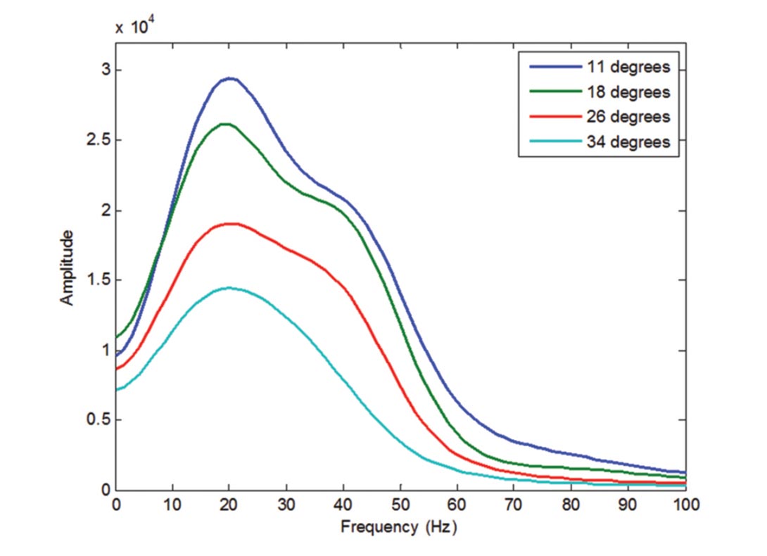
Consider the smoothed spectrum of four angle stacks used in an AVO inversion as shown in Figure 6. By assuming that the reflectivity series is random in nature with a white spectral signature, we can attribute all spectral character to the seismic wavelet. Figure 6 then represents an approximation for the amplitude spectrum of the wavelets where the difference in scaling at zero Hz is attributed to the background AVO response.

Note that as the incidence angle and hence the propagation distance increases, the higher frequencies are lost. This is characteristic of constant Q attenuation and therefore we can implement the associated properties to assist in the wavelet extraction process. Since the amplitude spectrum for each wavelet can be estimated, we simply need the associated phase spectrum, which can be derived using the fact that constant Q attenuation is necessarily coupled with minimum phase dispersion (Futterman, 1962).

Given that we can estimate the near angle wavelet of 11 degrees (we call this the pilot wavelet) using equation 2 with an acceptable amount of error, it can be represented by

where w is the frequency, A_p and φ_p are the amplitude and phase spectrum respectively and F^-1 is the inverse Fourier transform. The phase can subsequently be written as the combination of an unknown source signature phase term, φ^(ss) and a minimum phase component, φ_p^(mp) (Cho et al., 2010). This is represented by

where H represents the Hilbert transform. Assuming that the only attenuation mechanism is associated with constant Q, each separate wavelet can be written in a similar fashion as

where the subscript i represents the i^th higher angle wavelet. Now that we have a model to describe the phase evolution, we can attempt to estimate the phase spectrum of the higher angle wavelets by deriving a filter, γ_i that can be applied to the pilot wavelet. Therefore, we have

and the resulting filter is given by

The filter given by equation 9 can subsequently be applied to the phase spectrum of the pilot wavelet for an estimate of the phase spectrum of the higher angle wavelets. The resulting angle dependent wavelet is given by

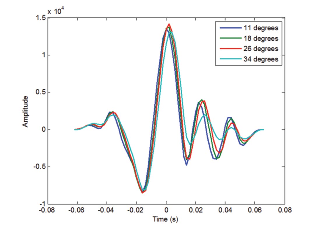
The proposed wavelet estimation therefore requires an initial estimate of the amplitude and phase spectrum corresponding to the pilot wavelet. Subsequently, the evolution of the phase for higher angle wavelets is achieved through a minimum phase filtering process which requires only the amplitude spectrum of the higher angle wavelets. The resulting higher angle wavelet is then constructed by the inverse Fourier transform of the corresponding amplitude spectrum and the filtered phase spectrum of the pilot wavelet. Figure 7 shows the resulting normalized angle dependent wavelets derived using the proposed methodology.

Conclusions

The errors associated with a least squares extraction of the seismic wavelet using synthetic shear wave velocities grow with an increasing angle of incidence. Given that a near angle wavelet can be extracted with an acceptable amount of error, a methodology for estimating larger angle wavelets was proposed. Using an estimate of the angle dependent wavelet amplitude spectrum and a constant Q attenuation model, we can evolve the amplitude and phase spectrum respectively to avoid the errors associated with the reflectivity calculations using synthetic shear wave velocities.

Acknowledgements

Many thanks to Meghan Brown for her constructive reviews and suggestions. The sponsors of the CREWES project are also acknowledged for their support.