Overview on the Fundamentals of Imaging

Introduction

The purpose of this paper is to review imaging, migration algorithms, and velocity model building. It gives an overview on the goals and techniques utilized in imaging of seismic data. The migration algorithms presented are based in the Gulf of Mexico but are applicable throughout the world. It is intended for those who are unfamiliar with seismic imaging or are not knowledgeable of seismic processing.

Imaging is the main goal of seismic processing. Traditional seismic interpretation involves identifying horizons, geological structures (faulting and folding), and seismic stratigraphy (onlap and downlap) in order to produce maps to understand the geology better. As we record seismic reflections we discover they are not where we record them in the subsurface due to:

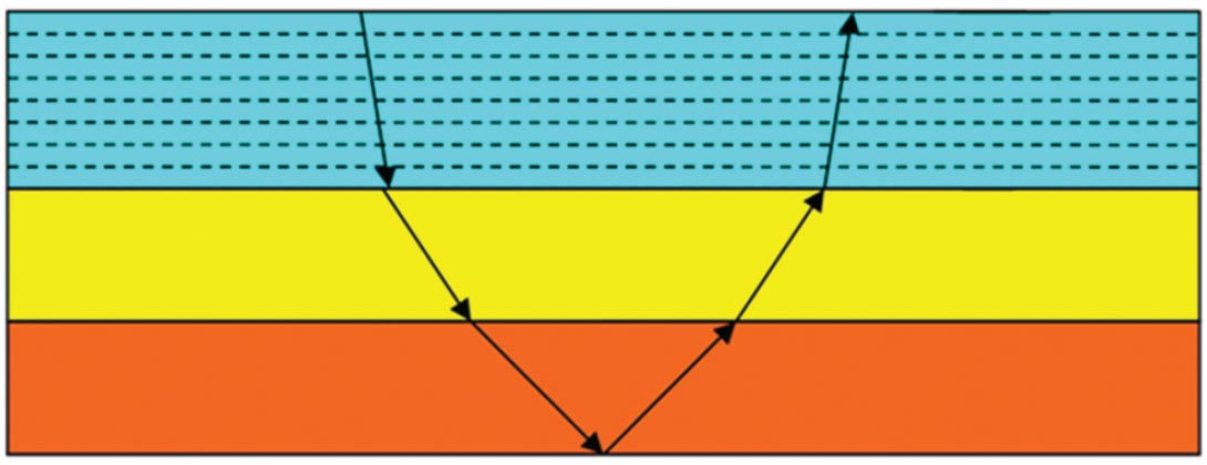
1. Snell’s law or ray trace bending is the change of the direction of the ray at the interface between two mediums or rock layers.

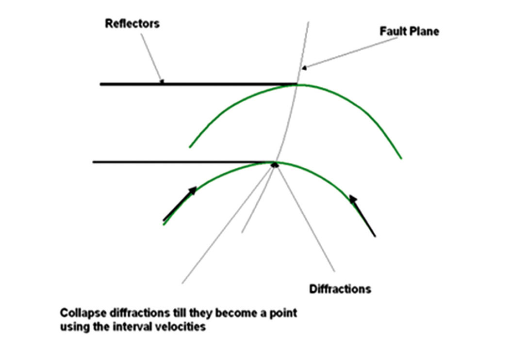
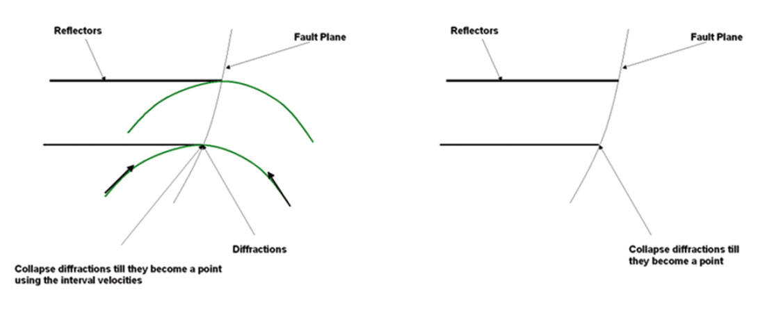
2. Hyugen’s principle describes the generation of diffraction hyperbolas we see in the seismic data from discontinuous reflectors. Each point acts as a point source which generates waves that travel spherically in all directions. With continuous reflectors the diffractions cancel, but when we have a discontinuity in the reflectors such as the edge of a geological fault the diffractions do not cancel out and we see them within the seismic data. The migration algorithms will collapse the diffractions to a point.

3. Pull up due to fast velocity layers or push down due to slow velocity layers;

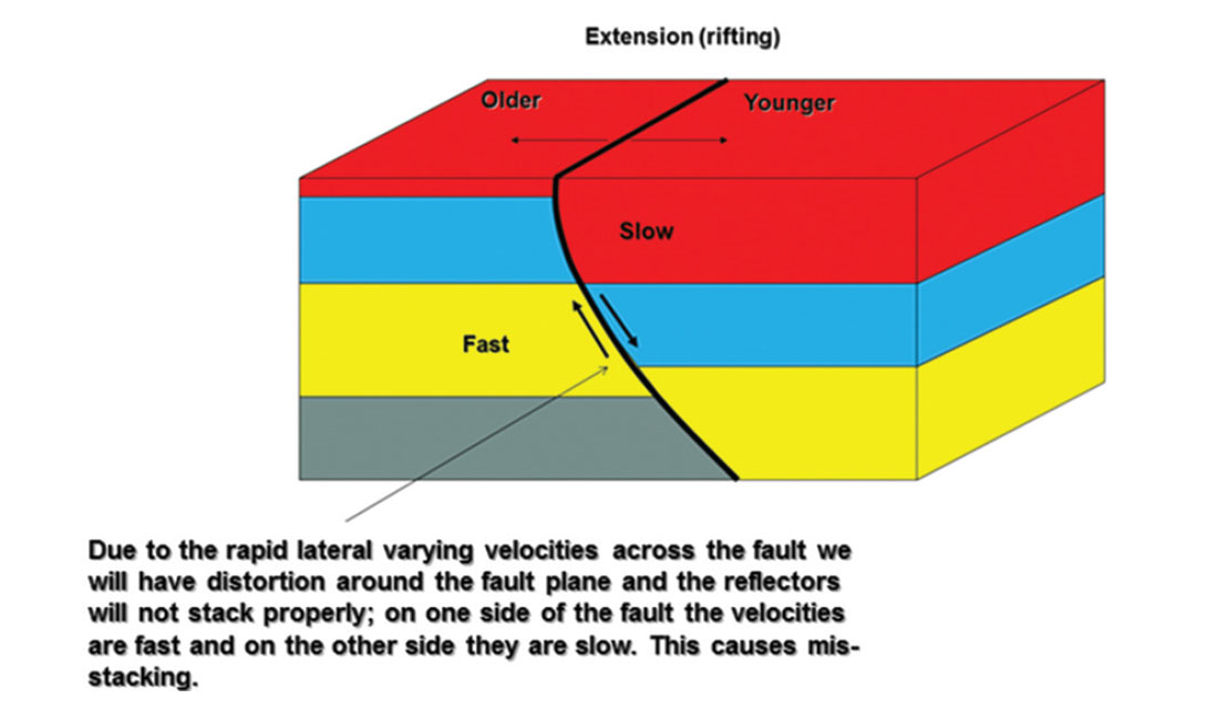
4. Fault shadows which are false structures in the seismic data generated by lateral changes in the velocity across the hanging wall and the footwall of a fault;

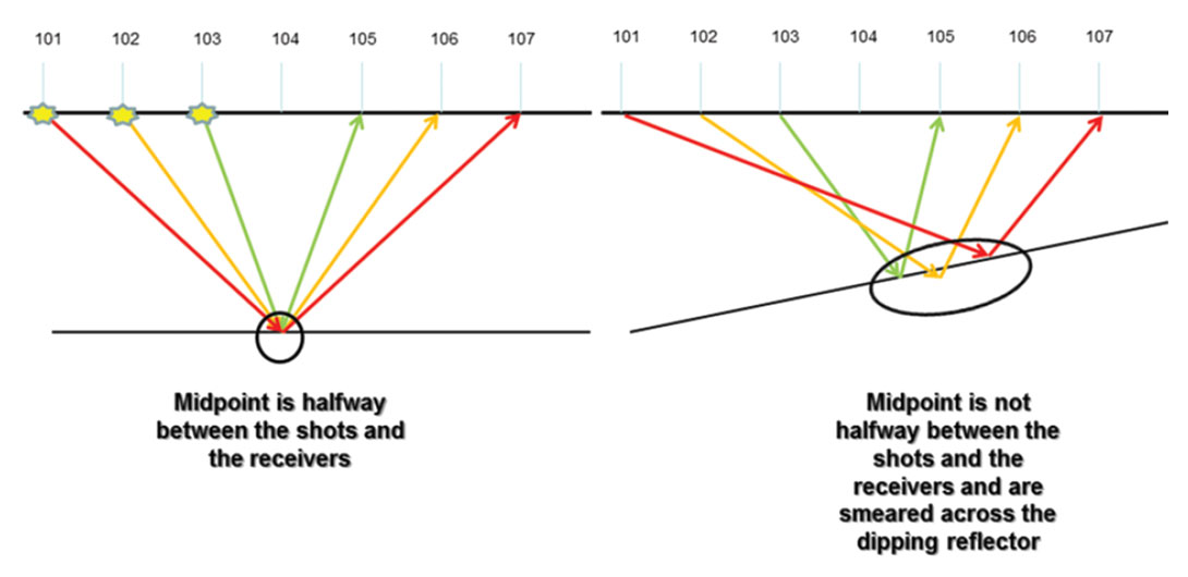
5. Smearing of velocities along dipping reflectors. The velocities for the dipping reflectors are different from the flat reflectors. This is a result of the Common Mid-Point (CMP) method assumption of a point being midway between the shot and the receiver on a flat reflector. If the bed is dipping then the CMP does not lie half way between the shot and receiver but falls across the interface as a smear. This causes the velocities between flat lying events and dipping events to be different.

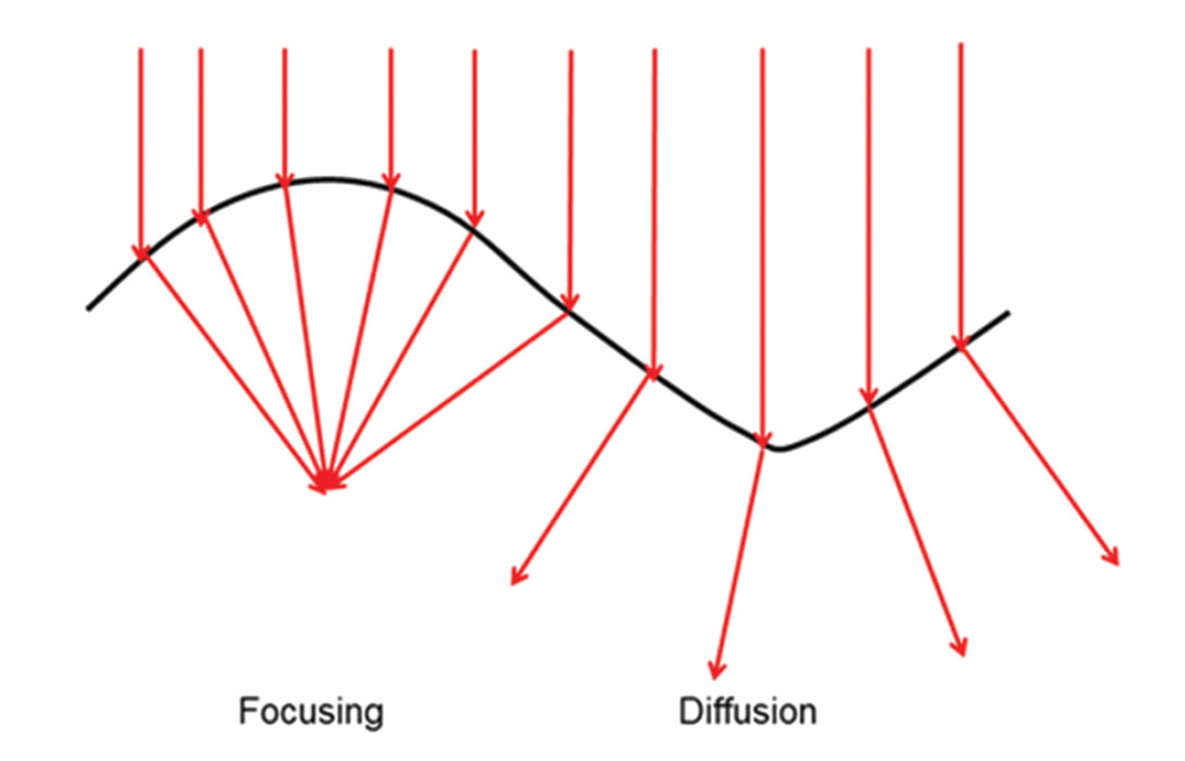
6. The lens effects caused by some rock layers such as salt which focuses some raypaths and diffuses others. This is why with subsalt we may have only small incident angles and it can be difficult to do subsalt AVO.

Seismic Design

The success of imaging is dependent upon the acquisition. When designing a 3D survey we need to understand the objectives of the prospect, the zone of interest, and we need to ensure that the area we are interested in can be imaged properly. This means we have enough data to migrate the zone of interest properly which is the the horizontal resolution of the seismic and is referred to as the Fresnel zone (Sheriff, 1996). The Fresnel zone is dependent upon the frequency and the velocity because it is based upon the wavelength (Sheriff, 1996).

When seismic data is migrated we are projecting the geophones through the earth until they are coincident with the reflector at which time the Fresnel Zone will have shrunk to a smaller circle (Sheriff, 1996). If the data and migration are 2D, then the Fresnel Zone will have only shrunk in one dimension and will still extend its full width perpendicular to the line. If it is 3D we shrink the Fresnel zone in all directions to a smaller circle (Sheriff, 1996). One benefit of 3D over 2D is the collapse of the Fresnel zone in both directions.

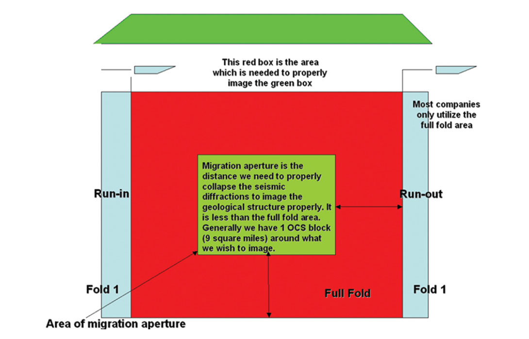
To properly image 9 sq. miles the minimum migration aperture indicates we need to acquire and process a total of 81 sq. miles with the 9 sq. miles being in the center. This data needs to be full fold data. The migration algorithms we utilize are based upon the principle of constructive and destructive interference. When we do not have full aperture we do not have full constructive and destructive interference so the data outside of the migration aperture may not be imaged properly. We should be cautious to drill on prospects on the edge of the data. Few prefer to output only what is in the full migration aperture while most want to image the full dataset to follow geological trends and to be able to possible new leads for future evaluation, but they must all be aware of the imaging limitations.

Wide Azimuth versus Narrow Azimuth Data

Having wide azimuths means we are sampling the structure in the earth in 360 degrees which allows us to illuminate or image the structure better. Wide azimuth data has the following benefits (Barley and Summers, 2007):

1. Improves the illumination of reservoirs beneath complex structures;
2. Better imaging and an ability to determine the orientation of fractures in azimuthal data;
3. Improves the signal to noise ratio;
4. Higher fold;
5. Better offset distributions;
6. Better azimuthal distribution;
7. Diverse sampling of noise;
8. Helps with multiple attenuation.

Conditioning Pre-Migration

In order to do proper imaging of the seismic data we must condition it properly. This involves removing noise and regularization.

Noise attenuation has become a major issue in the industry and it is felt that noise attenuation should be done in a series of steps removing the noise with trying to retain the signal. The goal is to remove any spikes within the data which will contaminate the migration by creating “smiles” or swings of the spike across several traces.

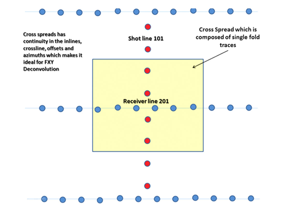
One common method of noise removal is FXY prediction filtering or FXY Deconvolution to remove the random noise on common offset planes. We can apply the FXY Deconvolution in different domains. With orthogonal acquisition we can utilize the cross-spread which is defined as all the receivers in a single receiver line which are listening to all of the shots in a single shot line. When we look at seismic data we can see the cross-spread is a regular, single fold, continuous 3D subset of the prestack wavefield (inline, crossline, offset, and azimuth) (Vermeer, 2007), which means that these spatial attributes vary smoothly from trace to trace (Vermeer, 2007). This is an ideal domain for noise attenuation.

Another issue we have with the seismic acquisition is where we have missing traces, infill and irregular fold. It is difficult to acquire a perfect seismic survey. We may also have poor sampling along one or more directions. Gaps and poorly sampled data cause migration artifacts because migration is based upon the principle of constructive and destructive interference.

Today there are more sophisticated methodologies to interpolate and regularize the seismic data such as 5D interpolation. 5D interpolation is interpolation in the inline, crossline, offset, azimuth and frequency domains. The 5D interpolation helps reduce migration noise and acquisition footprint within the seismic data. It fills in the small gaps, regularizes and provides better sampling of the seismic data which results in an overall better migration.

Migration

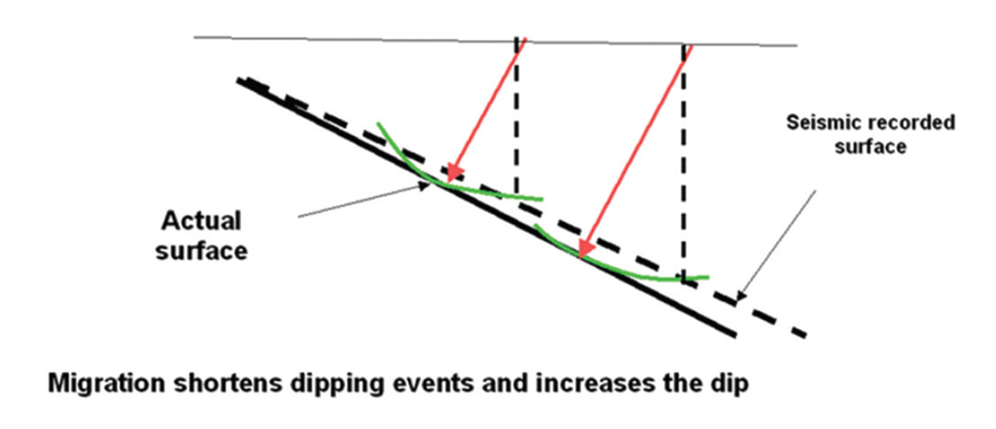
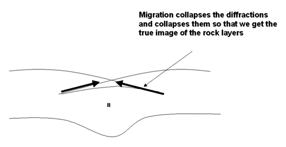
Migration is the process which the seismic data is properly placed in the subsurface by moving dipping events to their correct positions; collapsing diffractions; removing seismic bowties in the data; and increasing spatial resolution resulting in data that is more interpretable and coherent. Fault planes are visible and the seismic data appears to be similar to a geological crosssection. When we see diffractions and bow-ties still in the data we know that the seismic data has not been properly migrated.

Bowtie

One of the classical pitfalls of seismic data with is what is called “bow-tie” features, because they look like “bow-ties”.

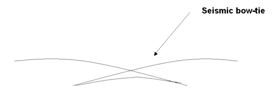
Before we collapse the “bow-tie” it appears at first that it will be two anticlines but in fact it becomes a syncline.

Post Stack Migration versus Prestack Migration

Migrations can be prestack or post stack. In the past it was common and economical to do Dip Moveout (DMO) stack + Post Stack Zero Offset Migration. DMO is a partial migration and not a full migration. It allows us to correct for smearing of CMP’s on dipping events and allows us to pick dip corrected velocities (figure 5B). The Post Stack Zero Offset Migration was then used to fully migrate the data.

We are now using the Post Stack Zero Offset Migration to create a fast track volume which is not AVO complaint that we can use to pick horizons that will be later overlaid onto the AVO Complaint Prestack Migrated Data.

With the development of AVO, better migration algorithms, faster computers, parallel computing, cheaper disk space and memory we have seen the rapid development of Prestack migration. Energy and Production (E&P) companies are utilizing 3D seismic data combined with Prestack Time migration, gather conditioning and flattening, and AVO to drill better wells. These companies are using AVO attributes and cross plotting in their exploratory data analysis (EDA) to illuminate potential prospects but not as a direct hydrocarbon indicator. Once an AVO is illuminated in the seismic volume the seismic gathers are visually interrogated to confirm the AVO and to insure it was not caused by processing artifacts such as multiples or non-flat gathers.

Geological Model Building for Imaging

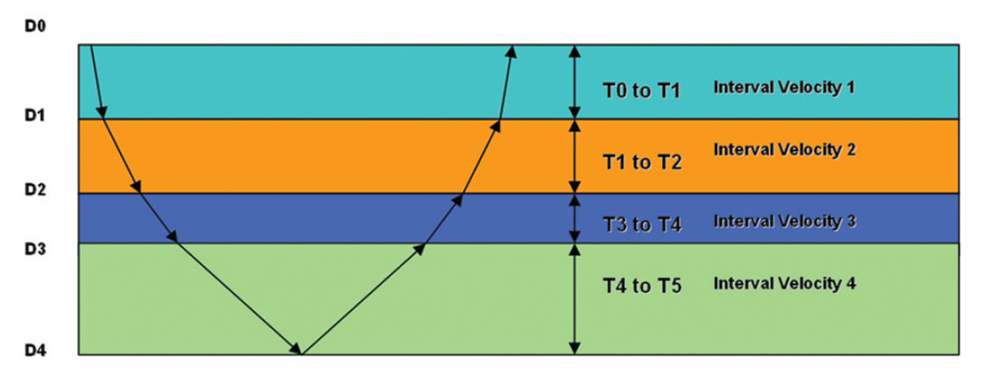
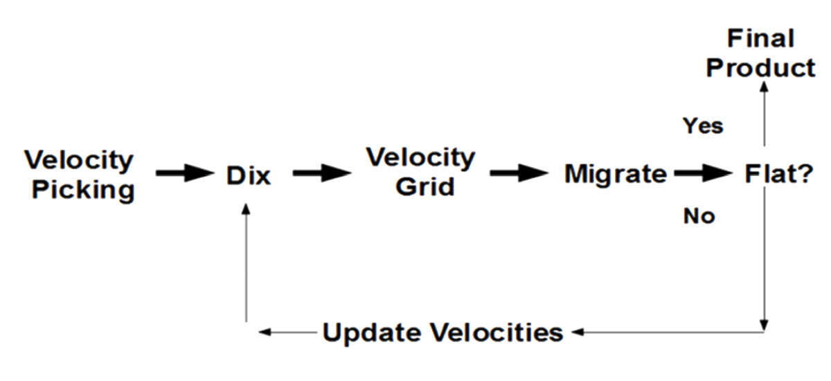
In the past velocities for time imaging velocities were chosen as the velocities that would flatten the gathers and produce the best stack. These velocities are referred to as Stacking velocities and are assumed to approximate root mean square velocities (V_RMS). We would then convert the V_RMS velocities to Interval velocities using the Dix (1955) equation:

Where:

V_INT is the interval velocity.

V_RMS1 is the root mean square (stacking velocity) for reflector 1.

V_RMS2 is the root mean square (stacking velocity) for reflector 2

t₁ is the travel time for the first reflector.

t₂ is the travel time for the second reflector.

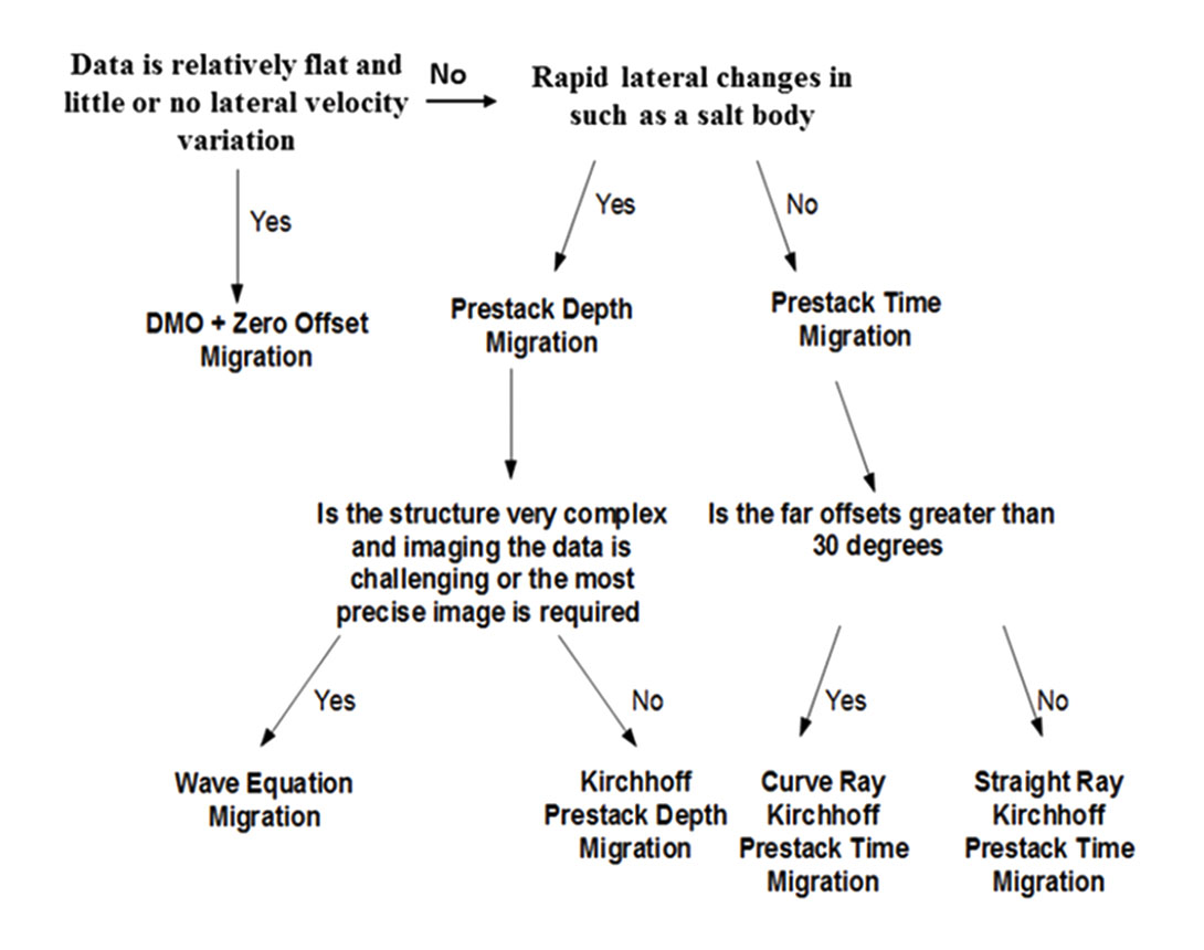
The interval velocities represent geological velocities. We found that with this technique of picking velocities only to flatten the gathers would produce at times physically impossible interval velocities. More effort is now being put forth to construct an appropriate velocity model for imaging incorporating seismic horizons, sonic logs, check shots, VSP’s, to provide as much geological velocity information as possible. The degree or intensity which we will develop the velocity field will determine if we will do a Prestack Time Migration or Depth Migration.

A rule of thumb is whenever there are rapidly-varying interval velocity variations occurring we require Prestack Depth Migration.

The advantages of time over depth are:

1. Depth is more computational expensive;
2. Depth is more sensitive to velocity;
3. Time migration sometimes adequately meets the seismic imaging needs to do the interpretation.

Some of the cases where Depth excels over Time are where we have a more complex velocity field such as:

1. Where we have a fault shadow issue. This is where there is false structures in the seismic data generated by lateral changes in the velocity across a fault (figure 4);
2. With complex geology such as salt domes.

Though Time migrated data is adequate for interpretation it may still have issues with velocity push down or pull up effects (Figure 3) which will affect our drilling. This can cause structural distortions of time-migrated images and render them inadequate for accurate interpretation of subsurface structures. Before we drill a well the Time Migrated data should be stretched to depth.

When depth stretching we should actually utilize a layer approach where we calculate the thickness of each layer to the T₁)*Interval Velocity /2. (T₂-T₁)*Interval Velocity gives us the thickness of the layer. We do this for all the layers in an accumulated approach. This approach is good if we have dips less than 10 degrees and a well behaved velocity field.

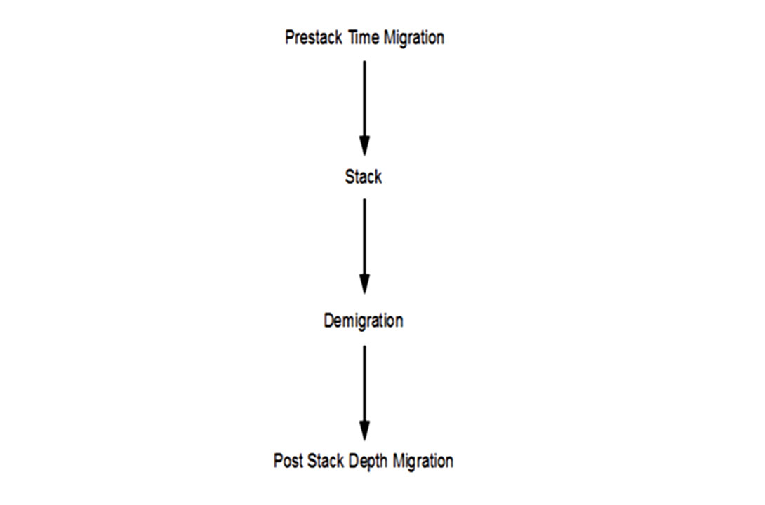
If the dips are greater than 10 degrees and the velocity field is not well-behaved, we need to use other techniques; one technique is taking the Prestack Time Migrated Stack; demigrating it; then remigrating it with a Post Stack Depth Migration as described in figure 14.

It is important to have a smooth velocity field with no sharp velocity boundaries when we do the depth stretching (Jones, 2009).

The issue with the Dix Equation is it may produce unrealistic and oscillating interval velocities. A number of approaches have been developed for inverse Dix transform, where a single erroneous value of stacking velocity does not easily corrupt the entire inversion. These methods are generally called constrained velocity inversion (Koren and Ravve, 2005) after Harlan’s (1999) algorithm that uses a least squares approach on the vertical velocity functions. Least squares takes a smooth function that approximately fits the data, throwing out the outliers. Further damping is applied to avoid unnecessary sharpness in the estimated interval velocities (Koren and Ravve, 2005). By applying these techniques, we are creating a smooth earth (velocity-depth) model. Smoothing and mapping is also done to generate a regular fine grid in space and time (Koren and Ravve, 2005).

Kirchhoff Time Migration

If we chose time migration generally we utilize the Kirchhoff Prestack Time Migration because:

1. It can handle irregular acquisition geometry as an acceptable input;

2. It has extreme flexibility in producing subsets of the output image volume such as common offset volumes. We can resort the common offset cubes back into Common Image gathers which is important for purposes of iterative residual velocity analysis, multiple attenuation and AVO analysis.

The disadvantage of Kirchhoff is that it requires a smoothly varying velocity field. This requires a reapplication of the velocities picked before smoothing to get the best stack or a repicking of velocities.

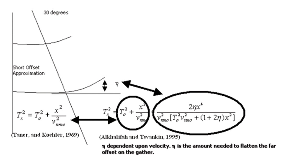
Earlier forms of Kirchhoff Prestack Time Migration were based upon a straight ray assumption, effectively assuming a locally constant lateral velocity. Later Curve Ray Prestack Time Migration was developed, which takes into account raypath bending due to changing velocity in depth (figure 1). The Curve Ray Prestack Time Migration allows us to image structures better and also it takes care of some of the anisotropy or hockey sticking we see on the straight ray or older Kirchhoff Prestack Time Migration. The Curve Ray Prestack Time Migration produces flatter gathers.

The Curve Ray Prestack Time Migration can be run in several ways:

1. Utilizing ray tracing;
2. Utilizing the fourth order moveout equation and ƞ which is good to about 18000 feet;
3. Utilizing the sixth order moveout equation and ƞ
4. Utilizing ray trace and ƞ. This takes into account true anisotropic effects similar to an Anisotropic Prestack Time Migration.

The ray-tracing based Curve Ray Prestack Time Migration can now handle lateral velocities and is becoming utilized for more complex geology.

Residual Velocities for Time Migration

Picked stacking velocities are spatially coarsely sampled typically on a 500mx500m grid. Because of this we lose the short wavelength variation in the stacking velocity field (Suaudeau, Le meur, and Hermann, 2002). This leads to poor stacking in areas where we have strong lateral variations in the seismic velocities. These areas require continuous velocities in order to flatten the gathers. Residual velocity error or inaccurate stacking velocities are a problem because non-flat gathers cause errors in the gradient (Spratt, 1987). This is why we developed automatic, high density, high resolution, continuous, velocities (AHDHRC velocities) in order to flatten gathers to provide a better stack.

AHDHRC velocities flatten the gathers up to about 30 degrees of incidence angle, which is equivalent to offset equal to depth. Beyond 30 degrees of incidence angle we have hockey sticking or anisotropy which results in a lowering of frequencies in the stack. In earlier days most mutes on seismic gathers were at 30 degrees of incidence angle. Now, we generally use a higher order moveout equation that utilizes a term referred to as  to flatten the gathers beyond 30 degrees.

Flat gathers also give a better, higher resolution stack response.

Factors which may affect the linear relationship between intercept and gradient are (Whitcombe et al, 2004):

1. Residual velocity;
2. NMO stretch (Keho et al, 2001);
3. Gain;
4. And overburden effects.

There may be some leakage of the intercept into the gradient (Hermann and Cambois, 2001; Cambois, 2002) for the AVO.

Types of Depth Migration

If the geology is complex we may then need to decide which type of migration to use. To decide, we need to understand advantages and disadvantages of each one.

Kirchhoff Prestack Depth Migrations (Raypath)

Similar to the previously advantages of the Kirchhoff Prestack Time Migration mentioned Kirchhoff Prestack Depth Migration has the following advantages:

1. It can handle irregular acquisition geometry as an acceptable input;

2. It can handle steep dips and turning rays;

3. It can handle anisotropy utilizing Thomsen’s ε and δ parameters;

4. Travel times can be calculated using three criteria:

Shortest ray path;

Highest amplitude;

First arrival

5. It has extreme flexibility in producing subsets of the output image volume such as offset cubes. We can resort the offset cubes back into Common Image gathers which is important for purposes of iterative velocity analysis and AVO analysis.

The disadvantage of Kirchhoff Prestack Depth Migration is:

1. It requires a smoothly-varying velocity field;

2. There is difficulty in accurately raytracing through complex velocity models;

3. It cannot accommodate energy that travels to an image location along more than one path (multipathing);

4. It does not accurately handle amplitudes.

Kirchhoff Prestack Depth Migration is a convolutional algorithm whereby we convolve a migration operator along the diffraction until the superposition of operators cancel everywhere but constructively add at the apex.

In order for Kirchhoff Migration to handle multipathing new migrations have been created.

Gaussian Beam Migration

Gaussian Beam Migration is between a Kirchhoff Prestack Depth Migration and a Slant Stack Migration (Hale, 1992). It is a generalized Kirchhoff migration that operates in the frequency wave number, as well as the time-space, domains (Gray, 2004). Kirchhoff Migration cannot accommodate energy that travels to an image location along more than one path (single raypathing). In Gaussian Beam Migration if several beams from the same source or receiver location strike the same image location, the Gaussian Beam Migration then accumulates these arrivals into that location creating multipathing naturally.

The Gaussian Beam Migration is done in two steps with the first step being local slant stacking (beams, each computed from small overlapping subsets of the seismic data) and the second step is being the imaging process itself. The Gaussian Beam Migration images along a particular beam which gives part of the total image and the total image is the sum of the contributions from all the beams.

The Gaussian Beam Migration can also be used to generate migrated gathers for velocity analysis.

Wave Equation Migration

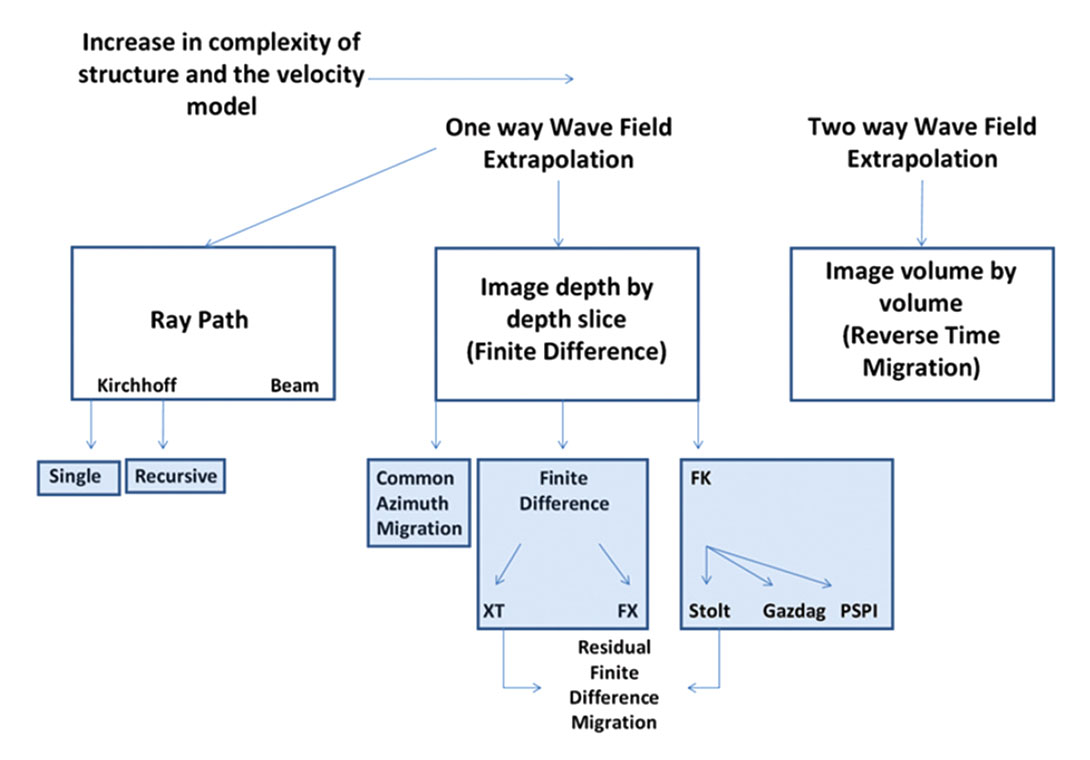
Wave Equation Migration (WEM) is a shot or common offset domain Finite Difference Migration and is advantageous wherever we have very strong lateral velocity variations, but has often historically struggled to image very steep dips. It treats amplitude simpler and unlike the Kirchhoff Migration, wave equation uses all the arrivals that are predicted by the acoustic wave equation allowing multipathing solutions. Wave Equation Migration is utilized in the most challenging situations for migration quality, or when the most precise results are required.

The disadvantages of Finite Difference are (Jones and Lambara, 2002):

1) Images the whole volume so requires a lot of computer nodes;

2) To obtain good dip response is expensive.

Finite Difference solutions of the wave-equation can be used to efficiently implement downward continuation. Downward continuation is the mathematical equivalent to lowering the receivers into the earth. If we have a diffraction hyperbola, as the wave field is continued into the earth the diffraction will collapse as the apex is approached, the migrated image is correct when the apex is reached.

There are generally two types of Finite Difference algorithms:

The Parabolic equation or the 15 degree approximation which images dips up to 35 degrees and is generally implemented in the time (XT) domain;

The “45° approximation” can image dips to about 65° and is usually implemented in the frequency (FX) domain or omega- X migration.

Common Azimuth 3-D Depth Migration

Common Azimuth Depth Migration is an efficient and accurate “wave equation” migration for narrow-azimuth seismic data, such as conventional marine streamer data. Common Azimuth Migration offers accuracy approaching that of Wave Equation migration, but at much cheaper cost. It can produce images superior to Kirchhoff migration in complicated geological areas such as regions of the Gulf of Mexico containing salt bodies.

FK Migration

Migration in the F-K or Fourier domain (Stolt Migration) is an important method since it is by far the quickest assuming constant velocity [v(z)]. It is accurate to 90 degrees and handles the amplitudes better (Li and Margrove, 1999).

Another migration implemented in the F-K domain is the phaseshift or Gazdag migration. This is a downward continuation algorithm similar to finite-difference methods except the downward continuation is carried out by a phase-shift in the FK domain. As originally implemented the method can handle only a vertically varying velocity. A phase-shift-plus interpolation or PSPI migration was later introduced by Gazdag to handle lateral velocity variations. This method performs several migrations with laterally constant velocities and interpolates the final migrated results. Depth migration and imaging of turning rays is also possible.

Residual Finite Difference Migration

The method exploits the steep-dip but constant velocity assumptions of FK migration with the dip-limited but lateral velocity handling characteristics of a finite difference migration. The data are first migrated with an FK migration using the lowest velocity found in the section (e.g. 1500m/s). The FK migration will partially collapse diffractions so the flanks are no longer as steep. A residual migration is then run with the finite difference method using a computed residual velocity which can vary laterally and vertically. It overcomes some of the issues we have with general finite difference migration and steep dips.

Reverse Time Migration

Reverse Time Migration (RTM) utilizes the full two-way wave equation, propagating both the source wavefield forward in time, and the receiver wavefield backward (or “reverse”) in time. This algorithm can properly image energy from all arrival paths, without dip limitation, in the presence of significant velocity variations, and in the presence of complex and overturned geologies. This allows RTM to provide extremely accurate image focusing without limitations, but at large computational costs.

Depth Velocity Model Building

Depth modeling is complex because when we change the interval velocity we also affect positions in depth. There are many issues with how we build the model for depth migration; it involves significant input from the interpreter as well.

Processing companies are spending their research and development on developing better methods and programs to update velocity models. The success of the depth project is dependent upon the velocity model.

Coherency Inversion

This technique is fast, and it involves no picking of seismic horizons, so it avoids the pitfalls related to interpretation. It is not very accurate for complex structures because there is no actual 3D migration of data involved, but merely a 1D perturbation of the local velocity field. It is used with horizon-consistent velocity analysis to construct the initial velocity model. It is a layer stripping approach, where the interval velocity is estimated layer-by-layer.

In essence we are creating ray-traced corridors for a range of perturbed velocities to produce semblances and we choose the maximum semblance by picking. The interval velocity is updated at this CMP location by simple vertical Dix inversion update.

This methodology assumes that we can accept a constant velocity perturbation within the ray bundle, and update the model point-by-point vertically.

Deregowski Loop

Deregowski loop is a vertical update that is based upon the assumptions of straight-ray and small-offset/depth ratio. It converts the depth residual into time residual and the velocities are converted to depth using the interval velocities obtained by a layer-stripping Dix equation. There are inherently two issues with Deregowski loop:

a) The results from the Deregowski loop are often unsatisfactory;

b) An error accumulation in depth is intrinsic to this process.

There are two ways to run Deregowski Loop:

1) Gridded where we output Common Image Gathers at the velocity locations and pick the velocities (the velocities do not necessarily follow horizons). To do this we need to understand how the velocities behave, such as estimating the compaction gradient, which commences from a given depth (usually the sea bed). The compaction gradient and the starting velocity are, in general, spatially variant;

2) Horizon picking where we can layer-strip which by freezing the interval velocities obtained by Dix in the shallower layers when a satisfactory solution has been obtained, and continue to pick the layers below. The issue with layer stripping is we introduce accumulation errors during the vertical update that proceeds from the surface downwards.

Tomography

Tomogaphy utilizes raypaths to correct for the residual velocity which accommodates for ray-bending effects. The interval velocities are not derived by Dix but by globally solving a linear system of equations (Zhou et al, 2003). This partially solves the problem of error accumulation intrinsic to the layer stripping process with the Dix formula as mentioned above. There are different tomographic techniques. In general tomography requires the knowledge of reference depth reflectors or time events. These locations are provided through the interpretation and picking of events on the stacked image before the tomography begins (Zhou et al, 2003).

Use of Interval Velocities in Interpretation

Seismic interval velocities can be overlaid onto the seismic section to help with the interpretation. Seismic interval velocities represent geological velocities and may indicate:

1) Geopressure zones where an increase in pore pressures creates a decrease in interval velocities;

2) Hydrocarbons which reduce the interval velocities;

3) Compartments within the data and help identify sealing faults;

4) Changes in lithology.

We can utilize interval velocities to aid us in the interpretation.

One of the issues with AVO is that when we have Geopressure we may have a false AVO response because the change in amplitude is not due to fluid content or lithologies but rather due to the grains being pushed a part because of the increased effective pressure.

Conclusion

This paper covered as an overview what is needed from seismic acquisition and seismic processing to help us image the seismic data properly. It showed that we can break seismic imaging into Post Stack or Prestack; Time versus Depth; and the algorithm we utilize depending upon the complexities of the velocity model. It discussed the importance of stretching the time data to depth because of issues such as pull-up or push-down. We should be wary of drilling on time data because of these issues.

It talked about the migration algorithms, velocity model building and how interval velocities can aid in the interpretation.

Dedication

This paper is dedicated to my father Lloyd Schulte who passed away this spring and was one of the reasons why I became a geophysicist.

Acknowledgements

This paper would not have been possible without David D’amico’s help in editing; Meghan Brown recommending it; and the support of those I work with throughout Talisman and within the Integrated Subsurface Solutions group. I also wish to thank my many mentors through the years who challenged me technically.