Past, Present, and Future applications of Geophysics in Oil Sands – Part 2

This paper is dedicated to Dr. Larry Lines (1949-2019), who was involved with seismic imaging and inversion, reservoir characterization, conventional oil and gas exploration, geophysical studies of heavy oil, oil sands, and monitoring effectiveness of steam assisted gravity drainage (SAGD), and who mentored us all. We also acknowledge the graduate students who worked on theses over the years with the University of Calgary Consortium for Research in Elastic Wave Exploration Seismology (CREWES) and Consortium for Heavy Oil Research by University Scientists (CHORUS), both groups which conducted research into application of geophysics in heavy oil.

Introduction

This is the second part of a two-part paper. This part of the paper explores some of the most recent advances in using seismic data for oil sands reservoirs. These are Time-lapse (4D) Inversion for SAGD; Predicting where Bitumen has been Liquified using PS-4D Seismic Data; 4D Time-Lapse Full Waveform Inversion for the SAGD Steam Chamber Imaging; 3D DAS FWI for the SAGD Steam Chamber Imaging; The role of Geophysics in Emission Reductions; Conclusions.

The goal of this paper is to look at the present and future work of seismic in heavy oil.

Time-lapse (4D) Inversion for SAGD

In time-lapse seismic analysis, seismic inversion combined with rock physics modelling is particularly useful to understand and interpret the changes in the elastic properties of the reservoir that result from changes in pressure, temperature, and fluids during SAGD operations. The SAGD method consists of steam injection in horizontal wells to heat the bitumen and reduce its high viscosity to increase mobility.

“In 4D seismic, seismic inversion combined with rock physics modelling is particularly useful to understand and interpret the changes in the elastic properties of the reservoir that result from changes in pressure, temperature, and fluids during SAGD operations.”

For oil-sands reservoirs that are thick and have been heated and produced for a longer time, updating the initial low-frequency models becomes particularly important to eliminate artifacts outside production areas and obtain more accurate magnitudes of property changes. Updating the low-frequency models could be realized using different approaches such as scaling the models based on horizon shifts (with an example shown later in this paper, from Gray et al., 2017), or using time shifts measured between the baseline and monitor survey (with an example from Reine et al., 2020).

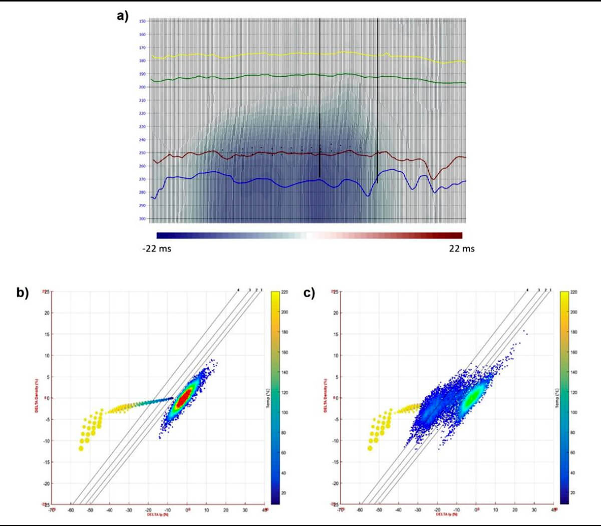
When converted PS data are not available, we can still update the S-wave initial model for the monitor by using rock physics modelling and PP time-shifts. Figure 12 shows an example from Reine et al. (2020), who calculated corrections for the density and P- and S-wave velocity models from the maximum injection conditions of pressure, temperature, and water saturation expected over the different lithologies.

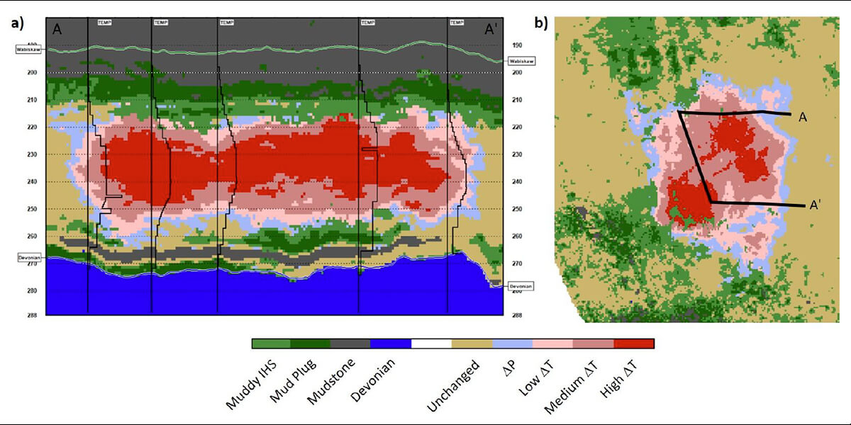
Figure 13 a) and b) show an example of facies classification of a non-uniform development of a steam chamber from a time-lapse seismic monitoring study within the McMurray reservoir (from Reine et al. (2020)). Often, intra-reservoir shale bodies act as barriers to steam propagation and impede the development of the steam chamber.

In this study, quantitative interpretation of baseline and monitoring PP data could directly image the fluid changes and flow outside the well areas by imaging and interpreting anomalies related to the SAGD steam chamber. Integrating the time-lapse inversion results with well rock physics data and other reservoir information, such as well logs, temperature, pressure, and core measurements, provided an excellent correlation between the seismic classes and the temperature logs.

Predicting where Bitumen has been Liquified using PS-4D Seismic Data

Recently Gray et al. (2017) demonstrated that liquid bitumen could be identified using the changes in seismic shear wave properties between surveys that can be identified in 4D seismic analysis that compares two PS surveys. The principle behind this is that the bitumen has a small amount of rigidity or shear strength in its natural state, making it a "quasi-solid" (Han and Batzle, 2008). Once the bitumen is heated to a liquid state, that rigidity, or ability to shear, goes away. In fact, the definition of the bitumen becoming a liquid could be its loss of rigidity. Because the rocks in oil sand formations tend to be unconsolidated, they have low levels of rigidity as well. Therefore, change from quasi-solid to liquid bitumen causes a large drop in the shear properties of the rock (Figure 14, green line). This large drop shows up in the PS seismic as a large change in the PS reflection amplitude, and a significant delay in the timing of the PS reflection below the liquified bitumen between the PS surveys taken before and after heating, leaving a large PS-4D seismic response (which geophysicists will call 3C-4D for 3-component – one component for pressure and two orthogonal components for shear). The reflectivity change can be detected using AVO effects, as described above, but the time delay cannot. The time delay is caused by the decrease in the shear properties, which includes decreases in the shear wave velocity through the entire liquified interval. Therefore, the converted, reflected S-wave moves significantly more slowly through the sand with the liquified bitumen, causing the seismic wave to arrive later. This time delay can be used to estimate the average slowdown through the 5 CSEG RECORDER MARCH 2022 sands with the liquified bitumen, which then allows the estimation of the average change in shear properties through that zone (Gray et al., 2017). This information can be incorporated into inversions, as described above. In particular, using AVO and PS data, geophysicists can estimate the change in S-Impedance (a function of seismic velocity, rigidity, and density), which is one of the most significant changes in the rock due to this liquefication (Figure 14). As can be seen in Figure 14, the change in shear properties seen by the inversion of the data after heating tell us whether the bitumen is liquid at any given point in the subsurface, if the shear impedance has decreased by 13%, in this case. If it is liquid, all that is required is a production well to produce the already liquid bitumen in that area. No further heating, i.e., no injection well, is required. Furthermore, the production well can be targeted to optimally produce the bitumen already liquified.

“The change in shear properties seen in the seismic inversion after heating tell us whether the bitumen is liquid at any given location in the subsurface.”

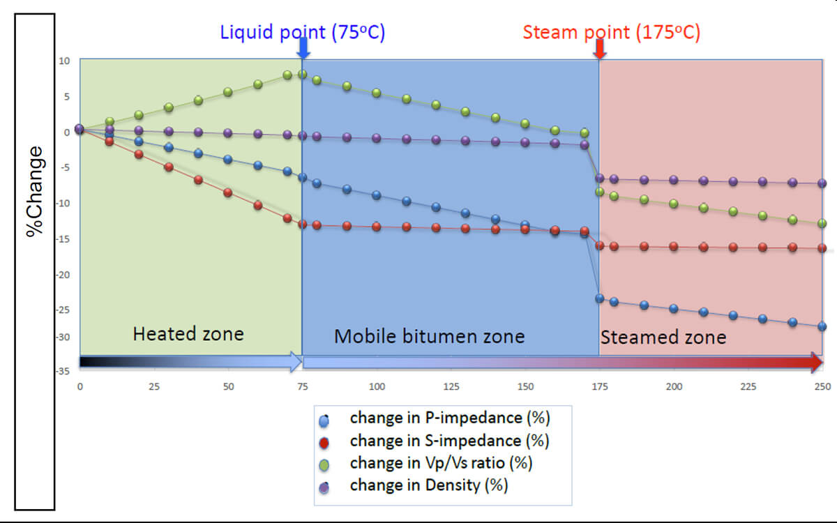
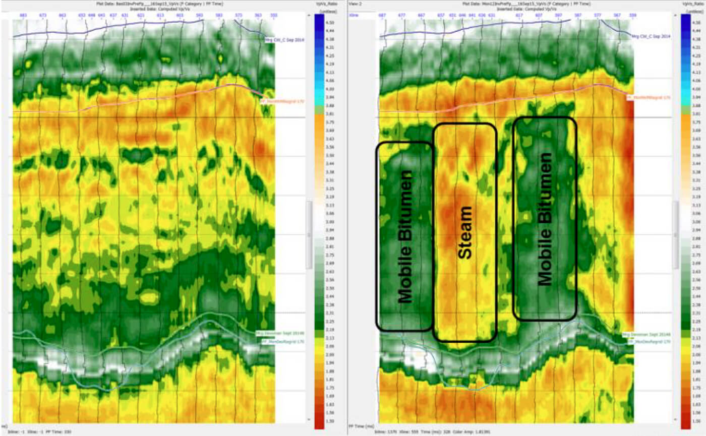
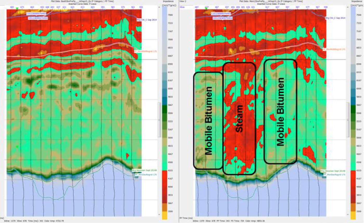
A geophysicist would likely interpret the location of the liquid bitumen by using PS-4D displays like the ones shown in Figure 15 and Figure 16. The images on the left of the figures are before heating, and on the right are after. Large decreases in P-impedance (Figure 14, red) show us where the bitumen has been replaced by steam. Large increases in Vp/Vs, caused by decreases in S-impedance (Figure 14, green), show us where the bitumen is liquid.

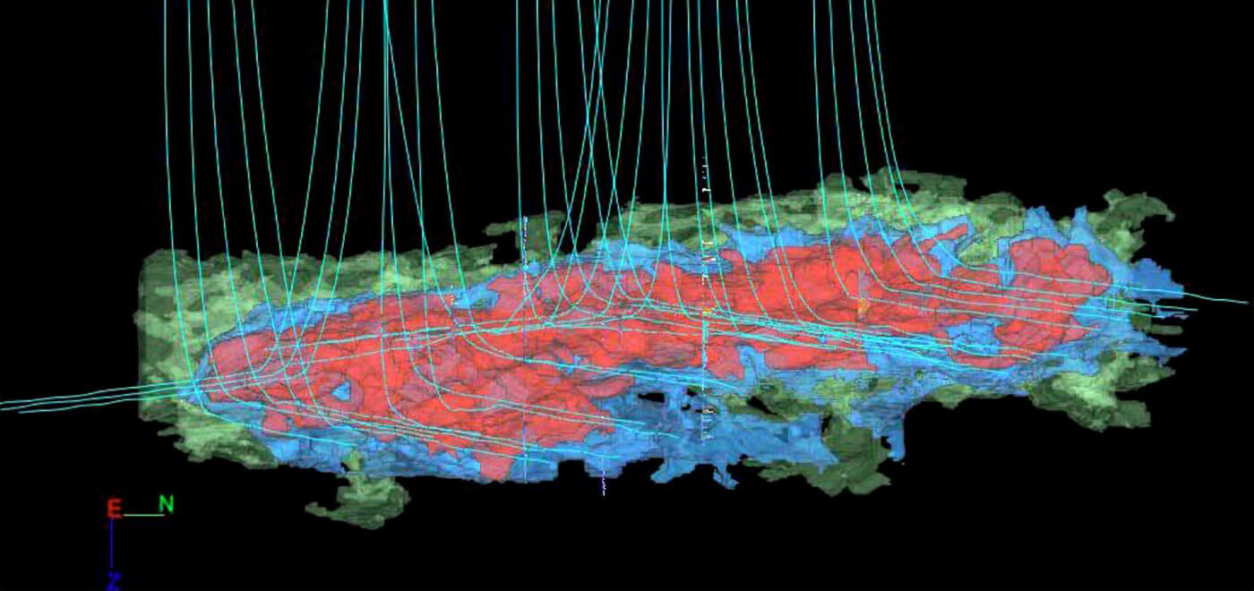
This interpretation can be converted in a manner similar to the facies inversion shown in Figure 13 or by using AI methods, as was done in Figure 17. Now the spatial distribution of the steam chamber (Figure 17, red), the spatial distribution of the liquid bitumen (Figure 17, red), and bitumen that has been heated, but is not liquid yet (Figure 17, green), can be displayed on a workstation and an infill well plan can be developed based on this display. Gray et al. (2017) found correlations of greater than 90% between the size of these distributions and the actual production of the reservoir, which suggests that these spatial distributions are reasonably accurate.

4D Time-Lapse Full Waveform Inversion for the SAGD Steam Chamber Imaging

During the SAGD process in oil sands production, 4D time-lapse seismic is widely used to monitor the steam chamber development (Lumley, 2001; Maharramov et al., 2016). Standard 4D seismic attributes, such as travel time delay and NRMS difference, are typically used to qualitatively interpret the thickness of the steam chamber and the location of the steam front. For most cases, it may be possible to pick a top steam chamber event on the stack reflection data. However, these interpretive attributes have difficulties to determine the geometry of the steam chamber in detail. The inverted velocity difference from the Full Waveform Inversion (FWI), which runs on the raw shot gathers with the possibility of a short 4D turnaround time, provides an efficient way for faster decision-making on production optimization and future well plans. Also, applying the FWI derived velocity model to create a PSDM volume can significantly improve imaging quality.

“The inverted velocity difference from the Full Waveform Inversion provides an efficient way for faster decision-making on production optimization and future well plans.”

Full Waveform Inversion initially emerged as an advanced tool for complex velocity model building (Crase et al., 1990; Warner and Guasch, 2014; Kotsi and Malcolm, 2017). The FWI-derived velocity model, coupled with advanced imaging algorithms, such as PSDM and RTM, can dramatically improve the subsurface imaging from extremely complicated structures that exhibit abrupt vertical and lateral velocity changes (Zhang and Zhang, 2011; Zhang and Huang, 2013). The oil and gas industry has seen very successful applications of FWI in different geologic settings, such as the complex subsalt targets in the offshore Gulf of Mexico. However, FWI has yet to extend its full potential to the land seismic data, especially the 4D time-lapse seismic surveys during the SAGD operation in Oil Sands areas. The application of FWI to the land seismic remains challenging mainly due to lacking low frequencies, limited offsets, high amplitude elastic waves, and source wavelet estimation. To mitigate these effects on the time-lapse FWI, the double-difference workflow (Bian et al., 2017) was applied using a cost function mainly targeting the baseline match and the waveform difference match between the baseline and monitor surveys.

The input data to the 4D time-lapse FWI algorithm are raw shot records (baseline and monitor) and an initial velocity model with an objective of deriving a final velocity model that would produce matching simulated shot records in both phase and amplitude using the finite-difference method. The output from 4D time-lapse FWI is the velocity difference volume between the baseline and monitor surveys. Velocity changes are a function of saturation, temperature, and pressure, with the greatest velocity change associated with a gas phase. As a result, the velocity difference between the baseline and the monitor surveys can be used for the direct interpretation of the developed steam chamber. The preliminary analysis of the inverted 4D time-lapse FWI velocity difference shows a very encouraging image of the steam chamber inside the reservoir, which is crucial for understanding the heterogeneity of the reservoir and future development plans. The inverted FWI velocity difference was validated with vertical well temperature logs, top/base steam chamber events from the reflection seismic volume, the time delay map, and the surface heave map (Feng et al., 2020).

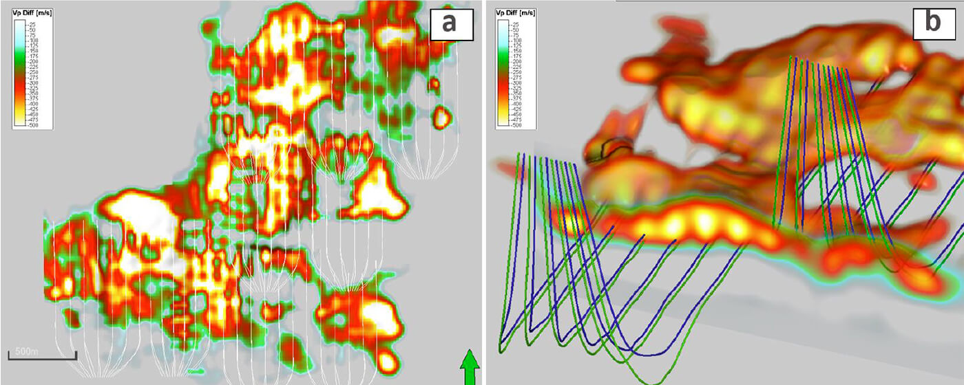
The validation and analysis of the FWI velocity model involve comparing with time delay map, vertical observation well temperature logs, and production data. The inverted FWI velocity differences agree with the temperature logs and have a good alignment with the horizontal trajectory. A map view of a depth slice of the FWI velocity difference at 16 m above the producers reveals a strong velocity drop along the horizontals (Figure 18a). A 3-D perspective view of a steam chamber geobody illustrating the velocity difference volume with horizontal and vertical slices over producing SAGD pads (Figure 18b).

3D DAS FWI for the SAGD Steam Chamber Imaging

Distributed acoustic sensing (DAS) using fiber optic cables is known in the oil and gas industry for monitoring the fluid inflow in wellbores. Full-waveform inversion, also known as full-wavefield inversion, is a data processing technique that has been employed in the oil and gas industry in seismic surveying, primarily in offshore 3D surveying of the complex subsurface structures. However, the application of FWI to 3D DAS on horizontal tubing-deployed fiber-optic cables is relatively uncommon. 3D DAS FWI is an innovative technology that could be applied to thermal bitumen projects as a potential alternative or complementary tool for steam chamber monitoring due to the low cost and operational efficiencies, and by using existing DTS cables as receivers, the surface impact is significantly reduced.

“3D DAS FWI is an innovative technology that could be applied to thermal bitumen projects as a potential alternative or complementary tool for steam chamber monitoring due to the low cost and operational efficiencies.”

The geometry of the 3D DAS survey is very different from conventional surface seismic programs in that the source points are on the surface, and the receivers are underneath the steam chamber target depth. 3D DAS FWI uses supercomputers and an advanced algorithm of FWI, processing the full wavefield including all the seismic wave types (refracted and diving waves, reflected waves, scattered waves, etc.) through the computer simulation to get a subsurface earth model in rich details in the depth domain. The input of the 3D DAS FWI workflow is the large quantities of the shot gathers recorded from the 3D DAS survey with a minor precondition of the data, and the output of the workflow are the subsurface rock properties, mainly P-wave velocity. The inverted P-wave velocity can be used as a direct indicator of the steam chamber.

A substantial amount of 3D DAS shot gathers were recorded on one SAGD pad where fiber-optic sensors were installed along each horizontal well for Distributed Temperature Sensing (DTS) measurements. There are six fiber cables with 100 m spacing. The fiber gauge length is 15 m, and the fiber channel interval is 1 m. The input data to the FWI algorithm are raw shot records with an objective of deriving a velocity model that would produce matching simulated shot records in both phase and amplitude. A Ricker wavelet with the center frequency at 35 Hz is used in generating the synthetics. The first breaks were picked to perform travel time tomography to get a starting model for the FWI.

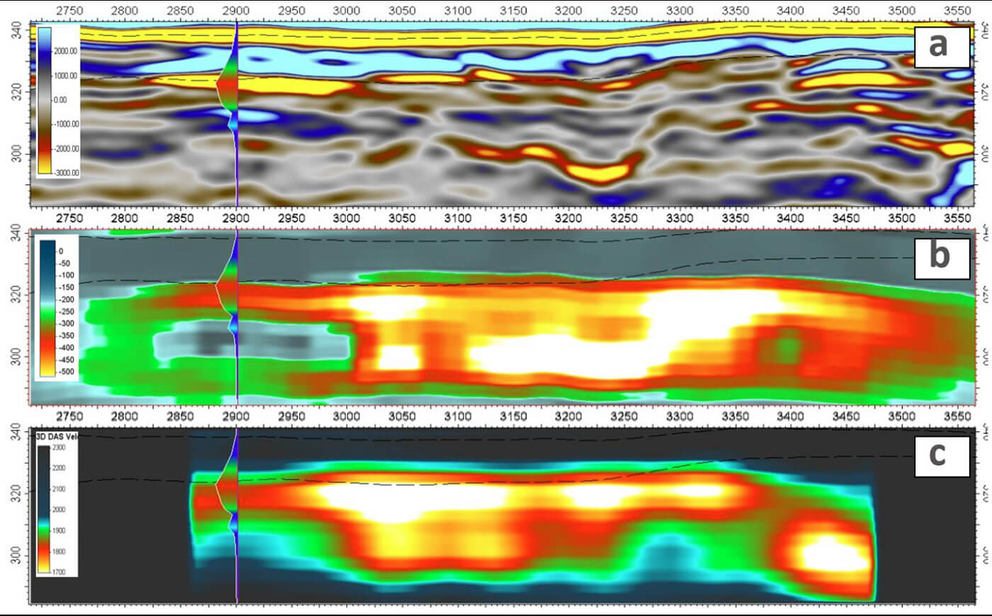
Although finer resolution of velocity could be achieved with a dense sampling along the horizontal direction, the inadequate illumination from the shadow zone in the 3D DAS survey due to the sparse fiber-optic receiver lines imposes challenges on 3D DAS FWI. The inverted velocity along the horizontals shows a higher resolution image in the inline direction compared with the crossline direction, which has an inadequate illumination. The preliminary analysis of the inverted 3D DAS FWI velocity shows a high-resolution velocity result where the illumination is highest. On the other hand, the 3D DAS FWI velocity at the edge of the survey shows some artifacts and poor results due to the inadequate illumination. The inverted velocity from the 3D DAS FWI is shown in Figure 19.

3D DAS FWI, as an innovative and cost-effective alternative to the conventional 4D time-lapse surface seismic, can deliver the velocity volume in the depth domain directly from the raw shot gathers with minor pre-processing of the 3D DAS shot gathers, which can result in a significantly reduced turnaround time to implement timely production decisions. To mitigate the illumination issue in the 3D DAS technology, DAS fiber on the surface or surface seismic can be used to resolve the illumination issue in the 3D DAS.

The role of Geophysics in Emission Reductions

Many countries, including Canada, have set goals for large reductions of anthropogenic GHG emissions. Canadian oil sands operations currently contribute about 25% to Alberta’s greenhouse gas emissions (www.alberta.ca/climate-oilsands-emissions.aspx). Therefore, Canadian oil sands companies announced the Oil Sands Pathways to Net Zero Initiative with the goal of reaching net zero emissions by 2050 (www.newswire.ca/news-releases/canada-s-largest-oil-sands-producers-announce-unprecedented-alliance-to-achieve-net-zero-greenhouse-gas-emissions-866303015.html).

Previous sections of this article have described the important role of geophysics in optimizing oil sands reservoir management, many aspects of which reduce the steam-oil ratios that are a proxy for reduced GHG emissions. Applications of geophysics in this way meaningfully contribute to reductions in GHG creation at the heart of thermal oil sands operations.

“Alberta is very well positioned for CO₂ storage and utilization at a large scale due to its geology and the technical expertise within the Alberta oil and gas workforce.”

One of the key, proven technologies towards achieving reductions in GHG emissions is through Carbon Capture and Storage (CCS), which may include Utilization (CCUS), e.g., https://royalsociety.org/-/media/policy/projects/climate-change-science-solutions/climate-science-solutions-ccs.pdf. This is a practical option to significantly reduce emissions from oil sands production. Carbon capture consists of the separation of CO₂ from operations emissions, and then utilization is converting the CO₂ to useful products or using it for enhanced oil recovery, as long as the produced oil has reduced carbon intensity. The latter has been proven, for example in the Weyburn Field, allowing the operator to be carbon negative (www.cbc.ca/news/business/bakx-ccs-enhance-whitecap-david-keith-1.5884107). Alberta is very well positioned for CO₂ storage and utilization at a large scale due to its geology and the technical expertise within the Alberta oil and gas workforce. For the Athabasca Basin, a challenge for implementing CCS is that the current regulations do not permit CO₂ injection and storage at depths of less than 1 km. This restriction is based on maintaining the CO₂ in a supercritical state for maximum storage efficiency and also for a high level of confidence that the CO₂ would not easily find a pathway to the ground surface and thus potentially contaminate potable groundwater or escape into the atmosphere.

Geophysics has a key role in CCS in terms of contributing to the Measurement, Monitoring and Verification (MMV) program to ensure security of storage and to map the CO₂ plume within the injection zone. Geophysical methods including seismic, electrical resistivity tomography (ERT), electromagnetic (EM), and gravity have all been used for monitoring CCS projects in Canada (e.g., Macquet et al., 2019). Seismic can also be critical in finding storage (porosity) in deep saline aquifers.

Conclusions

AVO techniques have a tremendous utility in the characterization of the oil sands reservoirs, despite the myriad complications affecting the seismic amplitudes (some of them discussed here). Experience has shown that one of the most robust strategies is integrating the seismic reflection data with AVO inversion and rock physics modelling. The key properties in the facies analysis are the density and Vp/Vs. They are lithology-dependent, with bitumen sands having higher densities and lower Vp/Vs and shales having lower densities and higher Vp/Vs.

In SAGD operations, time differences between baseline and monitor surveys provide useful information for updating the initial models for time-lapse inversion, which is necessary to obtain magnitudes consistent with the fluid, temperature, and pressure changes and to suppress the noise outside the heated areas. In the absence of converted PS data, we can obtain corrections for the interval values of Vp/Vs via rock physics modelling studies. In addition, even though the full-waveform inversion of DAS time-lapse seismic data cannot recover the shear information, and therefore the elastic properties, it has a wider frequency bandwidth and higher resolution and can complement the conventional seismic data.

Implementing CO₂ sequestration in the Athabasca Basin remains challenging. Through quantitative interpretation studies, we can obtain more accurate and detailed reservoir information, both laterally and vertically, which can help make better judgements, avoid costly mistakes, and significantly improve reservoir planning and economic outcomes.

Acknowledgements

We are thankful to the companies that provided the primary data and permitted sharing the results with the geoscience community. Draga Talinga would also like to acknowledge Sound QI Solutions for encouraging to share some of the case studies and Carl Reine for providing some of the figures used in this article.