Introduction
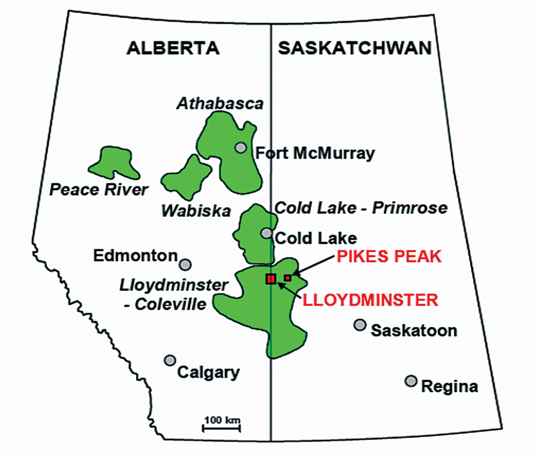
The Pikes Peak oil field is located 40 km east of Lloydminster, Saskatchewan (Figure 1) and produces heavy oil (12*API) from the Waseca sands of the Lower Cretaceous Mannville Group. Hulten (1984) provided a comprehensive geologic description for the Waseca formation in and around the Pikes Peak field. Over 42 million barrels of heavy oil have been produced at this site over the last 22 years. Presently, it is a significant oil field in Canada with a daily production of about 8000 barrels. (Husky Energy reports, 2004).
The primary objectives for this paper are to i) correlate the well logs, synthetic seismograms, and 3C surface seismic data from the Pikes Peak field, ii) analyze various attributes, in particular Vp/Vs, along the seismic line to delineate sandstone reservoirs, and iii) estimate the density and porosity in the zones of interest. Post-stack seismic inversion methods are used to estimate impedance values. Cokriging techniques are applied to integrate the sparse well measurements and the seismic data to estimate the density and porosity along the seismic line. With these methods, we have identified an interesting, yet undrilled, zone at the southern part of the seismic line.
Geology
The Pikes Peak heavy oilfield is situated in the east-central part of Western Canada sedimentary basin. The productive Waseca formation is located about 500 m below the surface and its thickness varies from 5 to 35 m (Figure 2).
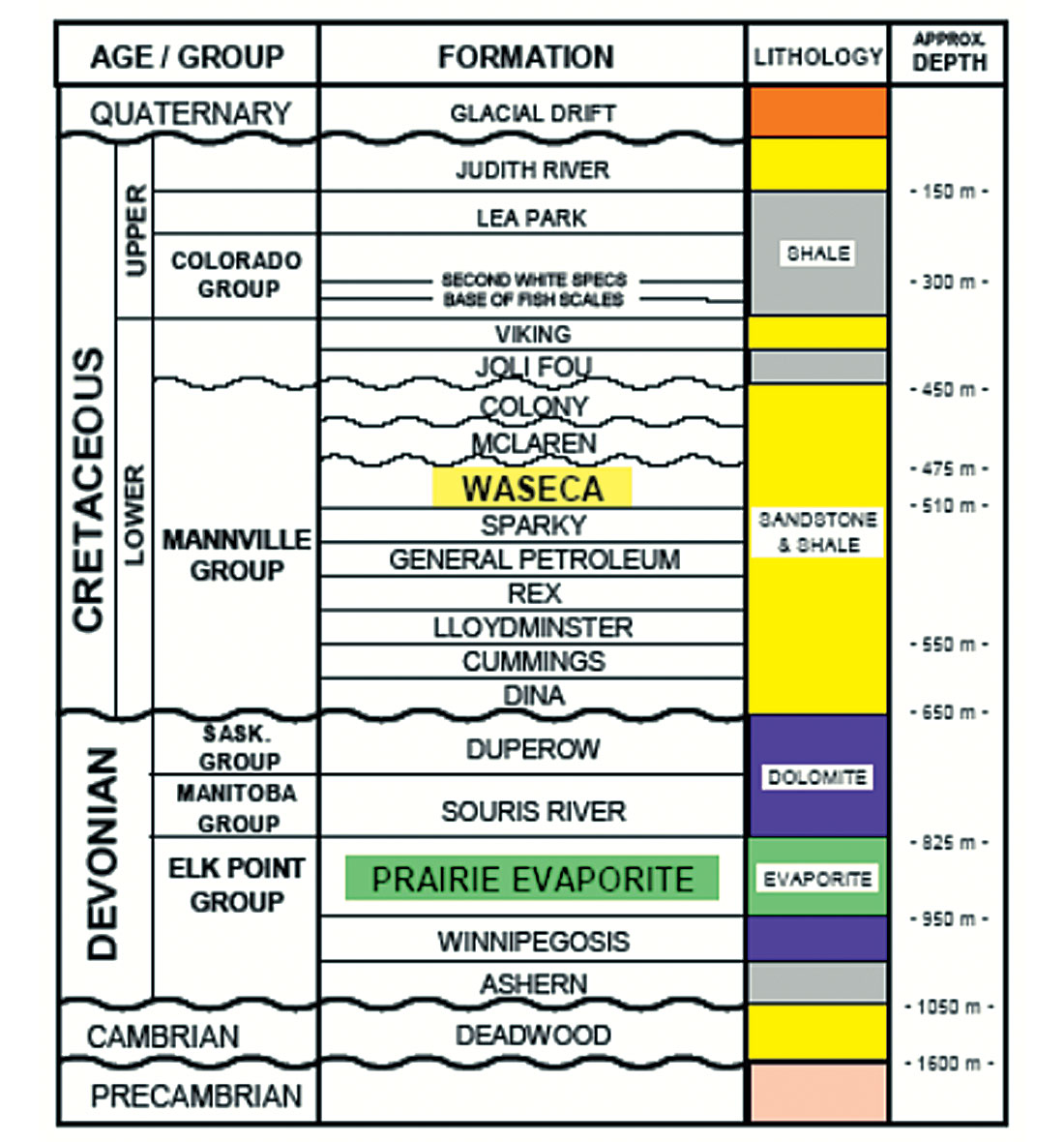
The top of the Precambrian basement lies at a depth of approximately 1600 m. There are essentially Devonian and Cretaceous formations above the basement. The dominant lithologies of the Devonian formation are limestone and dolomite, with the exception of the Prairie Evaporate, which consists largely of salt. The dissolution of this Devonian salt, played an important role in the formation of the hydrocarbon trap at Pikes Peak.
The 250 Ma gap between the Devonian and Cretaceous formations is the well known Pre-Cretaceous Unconformity. A mixture of sand and shale cycles were deposited above this Unconformity and they formed the Lower Cretaceous Mannville group. The Cretaceous strata are dipping largely to the southwest (Hulten, 1984).
The productive Waseca formation consists of three main facies. From the top to the bottom they are:
- sideritic silty shale unit;
- interbedded sand and shale unit;
- homogeneous sand unit.
The homogeneous sand, which is saturated with heavy oil, is the main target for development. This unit has the greatest thickness and continuity across the reservoir. The sands are well sorted, fine to medium grained. The interbedded unit is characterized with a lamination of sand and shale, which makes well log data “highly variable” in this part of the section. The upper shale unit plays the role of a cap in the hydrocarbon trap. It has low porosity and permeability, and creates a seal over the oil- or water-saturated sand. The trapping mechanism at Pikes Peak is considered to be both structural and stratigraphic: its stratigraphic component comes from the sealing shale unit and the structural component is determined by the dissolution of the Prairie Evaporite.
Well Log Correlation to Seismic Data
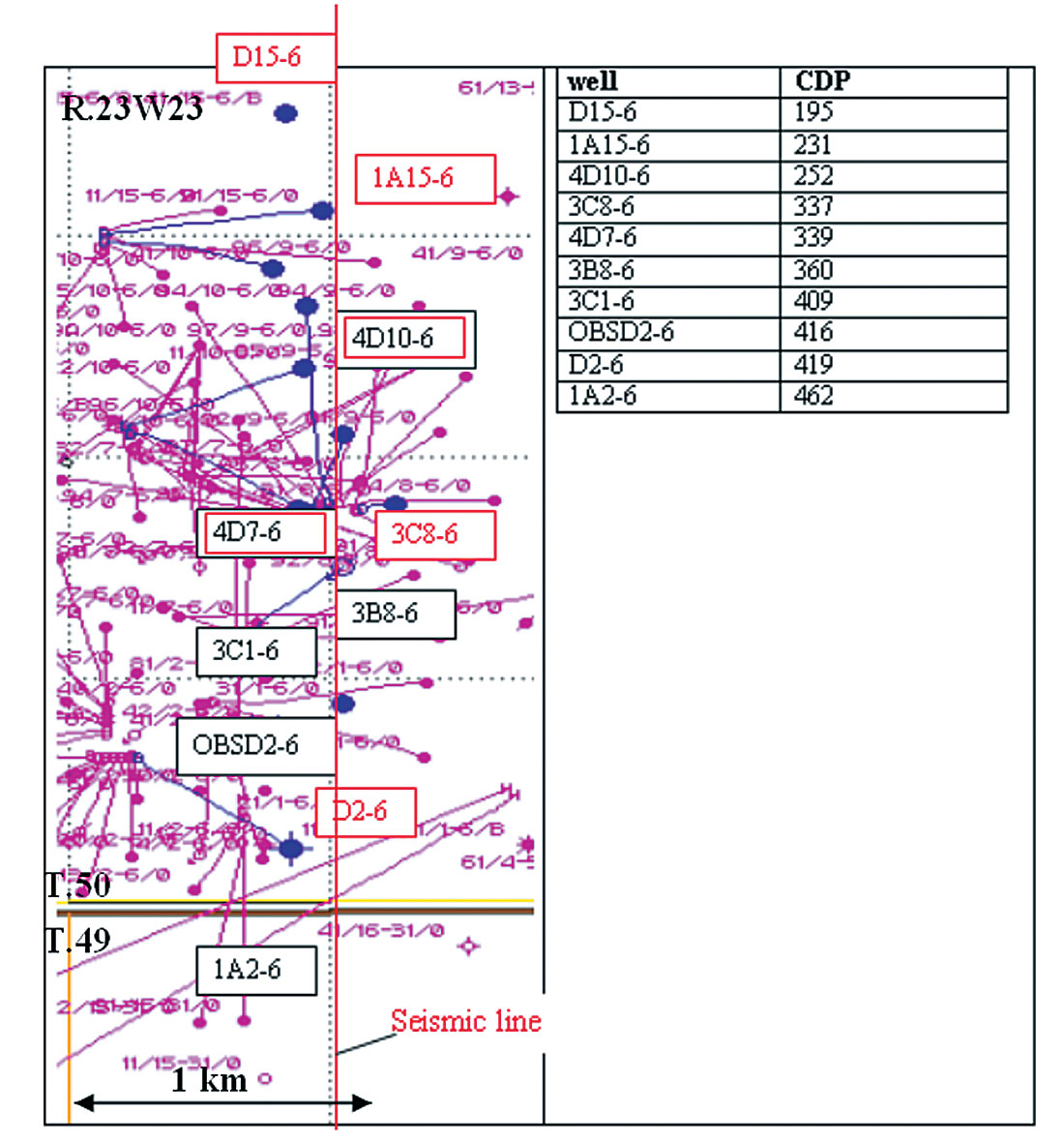
A three-component (3C) seismic line, acquired with a Vibroseis source, was collected in March 2000 by the CREWES Project and Husky Energy (Figure 3). This line was about 3.8 km long with a receiver interval of 10 m and a source interval of 20 m (Hoffe, 2000). Nine wells, closest to the seismic line (lying within 110 m of the 2D seismic line) were used for this work.
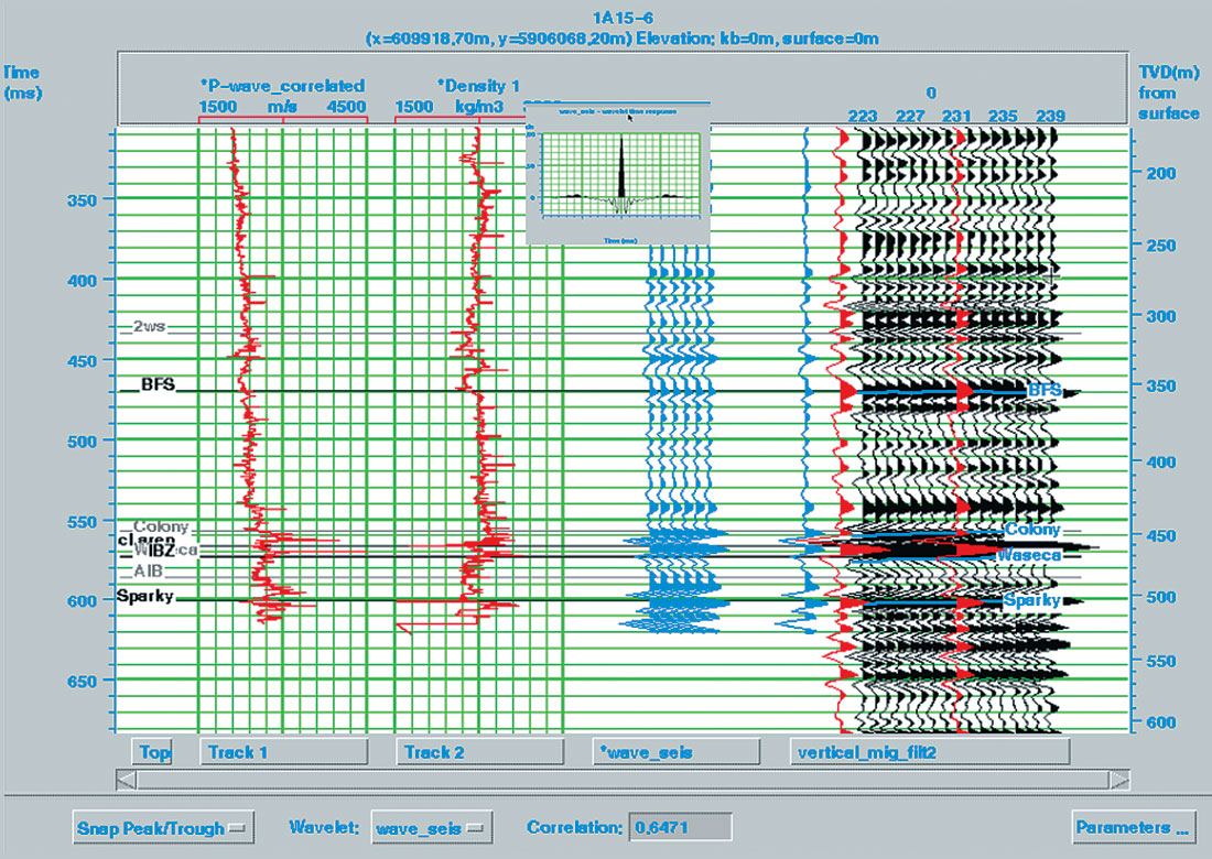
We begin the geophysical interpretation with the correlation of the well logs to the seismic data via synthetic seismograms. The logs, and resultant zero-phase synthetic seismograms, from well 1A15-6 are compared to the seismic data from around CDP 231 (Figure 4). We find a reasonable correlation in the data types (with a synthetic-surface seismic correlation coefficient of 64%).
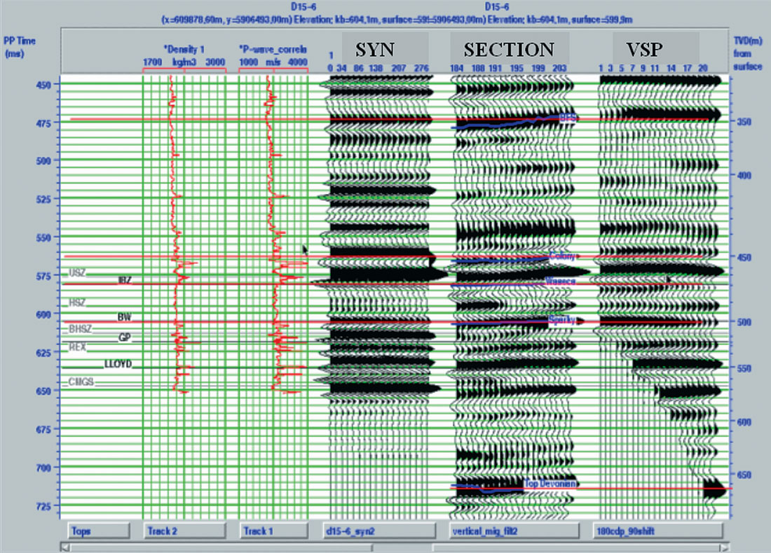
We can assemble the well logs, synthetic seismograms, VSP data, and surface seismic data into a composite plot, which helps with our interpretation (Figure 5). The VSP at Pikes Peak was conducted in the D15-6 well, which is fairly close to our seismic line. This well was chosen because it had not been used for reservoir steaming, and it passed through all the major area formations (Osborne and Stewart, 2001). The main events in the VSP correlate fairly well to the other data types.
VP/VS Estimation
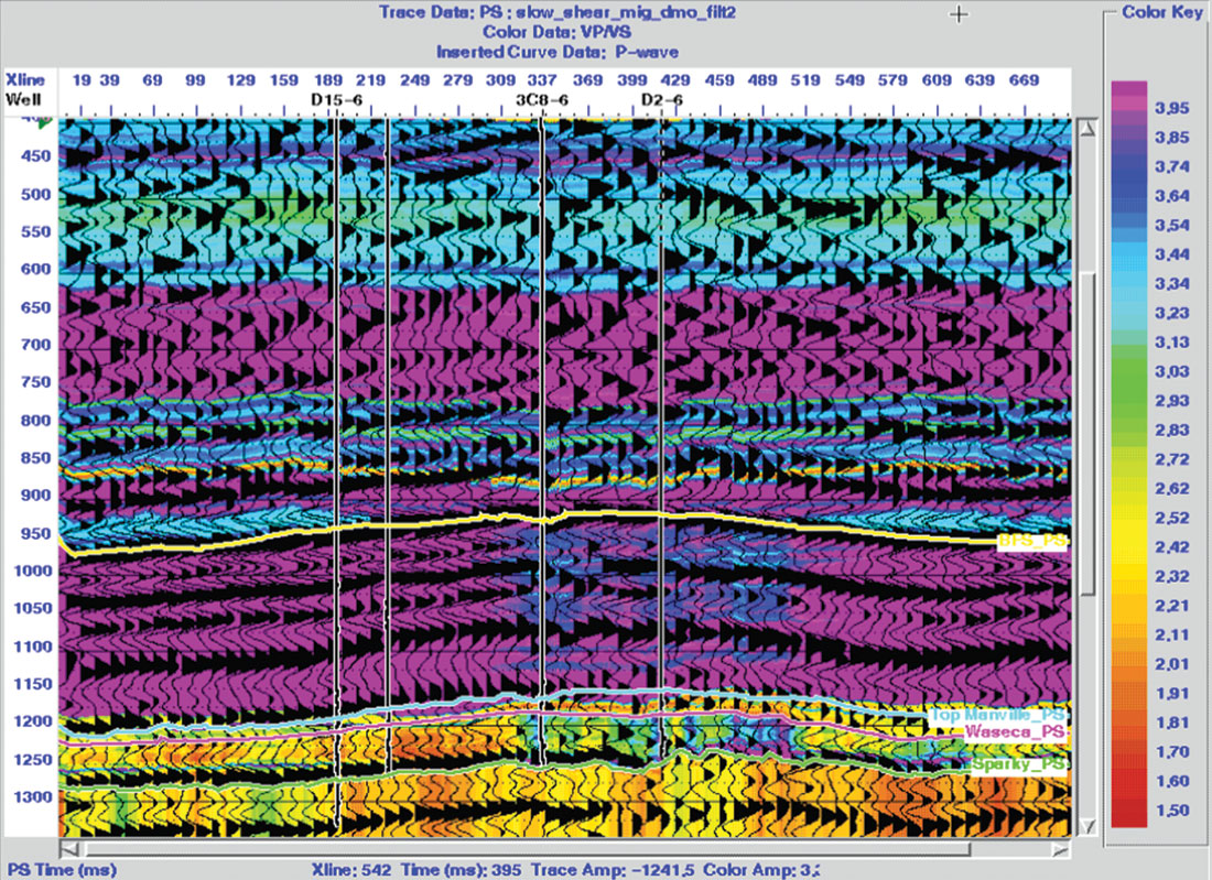
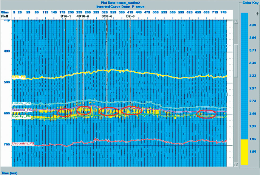
We follow the same procedure with well logs, synthetic seismograms, and correlation for the converted-wave (PS) section. The PP and PS sections are now tied together via the logs, synthetic seismograms, and linked horizons. We use the multicomponent seismic interpretation package, ProMC from Hampson-Russell to conduct parts of this interpretation. We next calculate a Vp/Vs value between the horizons and plot the color-coded Vp/Vs values for the line. This color Vp/Vs overlay is shown with the PS line in Figure 6.
The Vp/Vs calculation, based on interpreted time thicknesses along the seismic line, uses the following simple formula:

where ΔtPP and ΔtPs – are the time thicknesses between the horizons on PP and PS data sets, respectively.
The Vp/Vs values are quite high (around 4) in the Mannville shale and decrease in the productive sand interval (with the exception of coal layers). The coal layers typically have a higher Vp/Vs. In our case, this value goes up to almost 4 within thin coal layers of Waseca (at about 600 ms). The productive interval has Vp/Vs values of around 1.5 which is in reasonable accord with the well log data. The lowering of Vp/Vs in the vicinity of some wells may be caused by steam injection as well as better developed sand. Note that wells D15-6 and 1A15-6 do not exhibit any particular anomalies and they have not been recently injected.
The Waseca-Sparky time interval of almost 25ms correlates to a depth thickness of around 33 m. Thus, the Vp/Vs indicator represents an average across this depth interval.
PP Inversion
Inversion can be defined as a procedure for obtaining models which adequately describe a data set. (Treitel and Lines, 1994). For the seismic case, post-stack migrated data play the role of the data set to be inverted and the acoustic impedance is the desired property to estimate. Our zone of particular interest is the Waseca formation, which is going to be analyzed in terms of impedance anomalies. Since all inversion algorithms suffer some non-uniqueness, it is important to use external information to limit the number of possible models that agree with the input seismic data. Well log data provides the additional information to constrain our model – with the aspiration of making the inversion result more accurate.
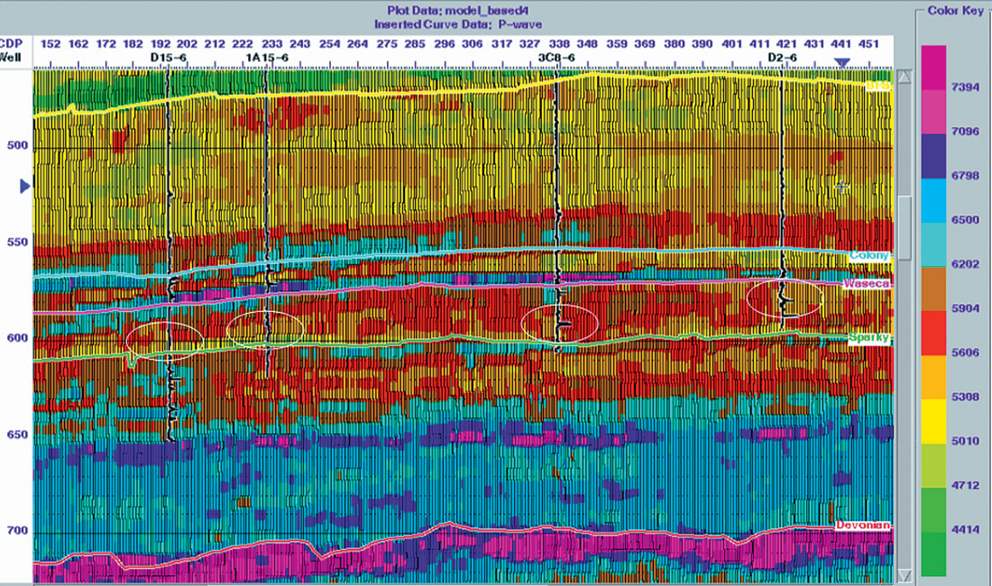
The initial geologic model was based on four sonic logs and four structural horizons. We experimented with a number of inversions, but one of the best results (as determined by continuity and correspondence to well information) is shown in Figure 7.
As expected, the impedance generally increases with depth with the exception of the productive zone (yellow through brown colors). The sand channel is indicated here as a low impedance anomaly.
PS Inversion
We undertook an approximate PS inversion that was similar to the PP inversion flow with the difference that the initial model was created using an S-impedance. Since we only had one S-wave sonic at Pikes Peak, it was used to construct the initial model. PS horizons in PP time were also included into the model.
The result of the model-based inversion with the corresponding well is shown in Figure 8. The productive formation here is recognized as an impedance increase (as opposed to a decrease in the PP case).
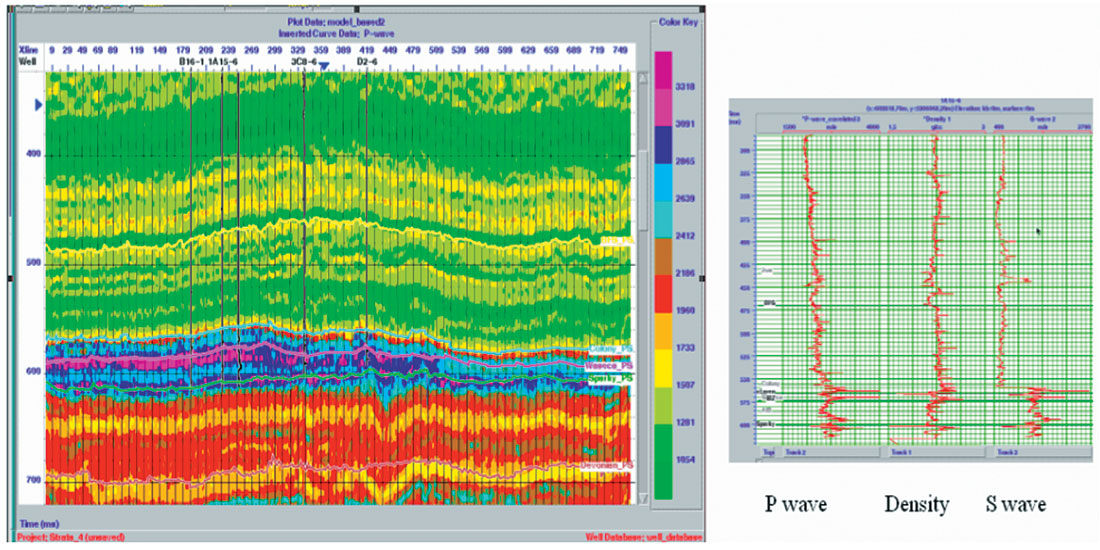
We can see a considerable increase in S-wave velocity in proximity to and through the Waseca formation (Figure 8, right). We now have inverted PP and PS data and can take the ratio of them to determine a Vp/Vs section (Figure 9).
All values lower then 1.95 are plotted in yellow (and all above in blue) to emphasize the anomalies and relate them to the well locations. We can observe some similarity between this image (from amplitude inversion) and Figure 6 (from time thicknesses). The productive formation is recognizable on both sections as having low values of Vp/Vs.
Density and Porosity Prediction
Mapping the physical properties of a reservoir is important for assessing and developing its hydrocarbon content. The Pikes Peak heavy oilfield is a heterogeneous reservoir, so we employ geostatistical methods to predict the rock properties between drilled wells. In this paper, we attempt to predict the density logs along the seismic line using multi attribute analysis.
Our aim is to find an operator that can predict the density logs from the neighboring seismic data. The desired operator can be estimated by analyzing different seismic attributes. Geostatistical methods sometimes use external attributes to improve the final prediction. Since we have two inverted datasets (for PP and PS data), it might be helpful to use one of them as an external attribute. We first use the PP data alone to calculate attributes (Figures 10 and 11).
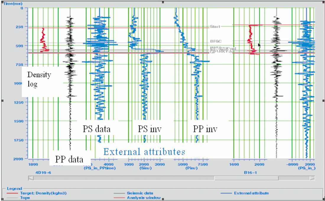
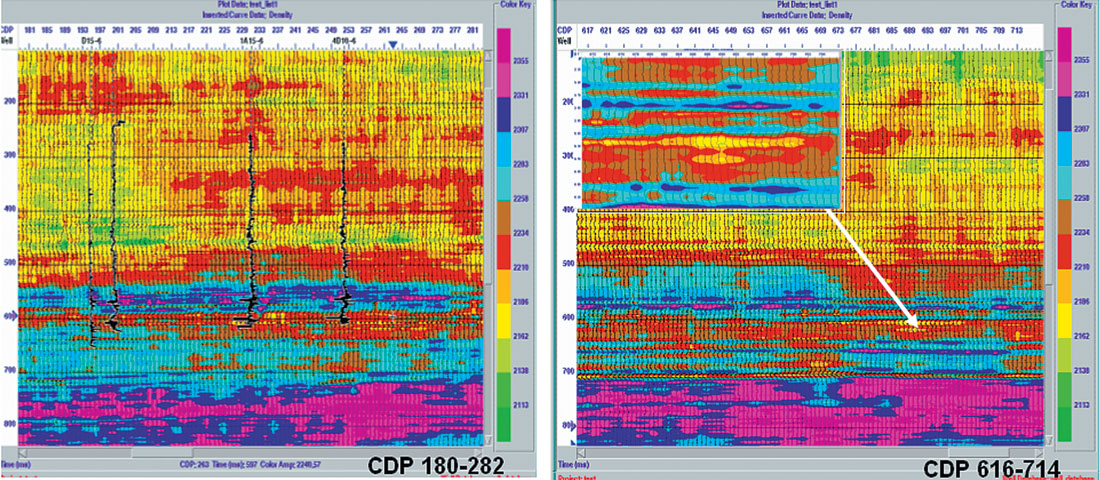
Table 1 shows the list of attributes selected by the step-wise regression as the best predictors of density. Each row includes all the attributes above. (Row 1 – best single attribute, 2 – best pair, 3 – best triplet, etc.) The corresponding training and validation errors are given in kg/m3.
| Target | Final Attribute | Training error | Validation error | |
|---|---|---|---|---|
| Table 1. Multi-attribute list with corresponding errors. | ||||
| 1 | Density | Amplitude Weighted Cosine Phase (inversion) | 70.75 | 71.38 |
| 2 | Density | Derivative | 69.01 | 70.60 |
| 3 | Density | 1/(Slowness) | 67.04 | 69.52 |
| 4 | Density | (inversion)**2 | 65.49 | 68.42 |
| 5 | Density | Quadrature trace (inversion) | 63.98 | 67.67 |
| 6 | Density | Amplitude Weighted Frequency | 62.75 | 67.02 |
| 7 | Density | Integrate (inversion) | 62.09 | 68.11 |
| 8 | Density | Cosine Instantaneous Phase (inversion) | 61.50 | 68.04 |
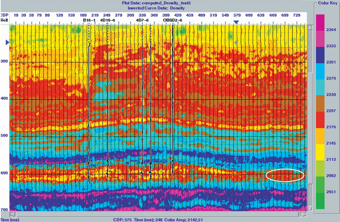
We apply the best 6 attributes to the seismic data to predict the density (Figure 11). In this case, geostatistical methods seem to help us to predict the density between the drilled wells. The productive zone here is seen as a density decrease at about 600 ms (red and yellow colors). If we view the southern part of the line, a density anomaly is observed between CDPs 685 and 700. This low density zone also correlates with a low impedance anomaly on the PP impedance section. No wells have been drilled yet at this interesting location.
We have also attempted to predict density using PS data as the internal seismic attribute, PP data, PP and PS inversions as the external attributes. The result is shown in Figure 12. Again, we see the density decrease in our zone of interest.
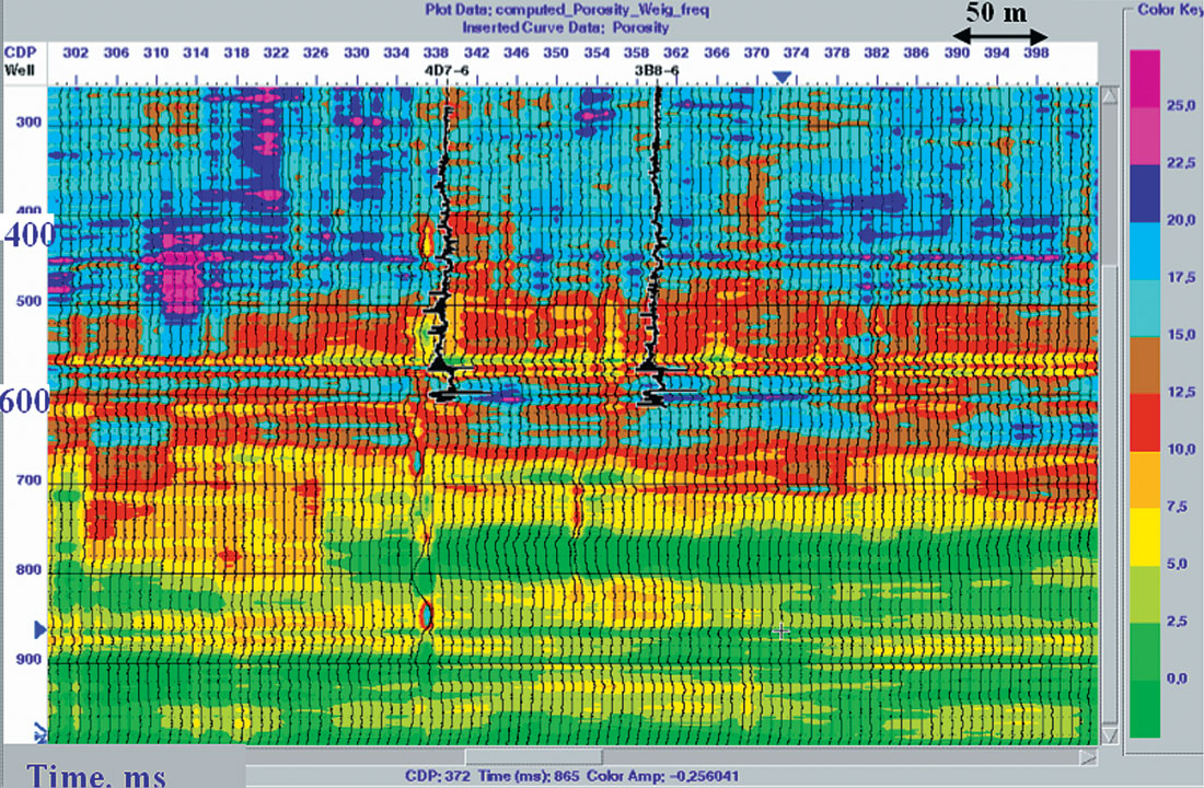
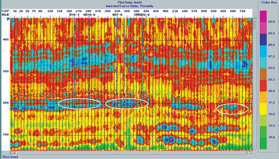
In addition to density, we can attempt to predict porosity. We first calculate porosity logs from the density logs assuming a sandstone matrix. We then geostatistically associate the seismic attributes to this porosity information. The results are shown in Figures 13 and 14. We note porosity values in the 15%-30% range in the reservoir interval.
Conclusions
The integration of well logs and multicomponent seismic data has been described in this paper. In the Pikes Peak case, the productive zone is associated with low Vp/Vs values as determined from PP and PS seismic data, inversion, and geostatistics. There is a considerable Vp/Vs decrease, from over 4 to less than 2, in the lithology change from shale to sand.
PP and PS impedance sections have been created and analyzed. The top of the productive interval is interpreted as a P-impedance drop and S-impedance increase . Inversion and other attributes have been used to predict the density and porosity along the seismic line. The productive zone has been characterized as a density decrease on logs, seismic data, and geostatistical estimates. Porosity increases in the zones of interest. A fascinating, and as yet undrilled, anomaly has been determined in the southern portion of the seismic line.

Acknowledgements
We express our gratitude to the sponsors of the CREWES Project at the University of Calgary for supporting this work. We are particularly appreciative of the assistance of Husky Energy Inc., in particular Larry Mewhort, for their considerable help in this project. We also thank VeritasDGC and Hampson-Russell for their ongoing software support.


Join the Conversation
Interested in starting, or contributing to a conversation about an article or issue of the RECORDER? Join our CSEG LinkedIn Group.
Share This Article