Quantitative Interpretation Part I: Method

Summary

Recent advances in drilling and completions technology, economics, and in our business model have been profound, and are overwhelmingly concerned with a quantitative description of material properties, stress, and azimuthal properties of our reservoir and its bounding materials. Surface seismic data can provide estimates of many of these variables, but has tended not to be used to its full extent because of an historical lack of quantitative orientation from geophysicists working at oil and gas companies. There are many reasons for this unfortunate deficiency, not the least of which is the phenomenal pace of change in the new business model driven by the exploitation of tight reservoirs. We must address these changes in business and engineering technology by embracing quantitative methods and get deeper into the fight to cost efficiently develop these tight resources. A number of recent publications have begun the process of addressing the need for quantitative approaches. This paper is meant to support the previous efforts and encourage the work yet to be done on this subject. We will describe what we mean by “quantitative methods”, their history, their value, their weaknesses, and why they are not only essential to tight reservoirs, but to all our efforts in effectively describing the earth. Specific examples of quantitative interpretation will be given in part II.

Introduction

The interpretation of minute waves of pressure into meaningful estimates of earth properties is a pursuit that is at once complex, uncertain, scientific, non-unique, analytic and artistic. This effort is rapidly evolving because of the current and growing need for more information relative to the exploitation and development of tight reservoirs. The multistage fracture stimulation required of these unconventional reservoirs has led interpreters to seek geomechanical properties in addition to lithologic and fluid estimates. This completions technology is so critical to the pursuit of tight reservoirs, that its application has essentially driven this element of oil and gas business. Some geophysicists have lamented that the oil and gas industry has minimized their importance in favour of engineering, that the art has gone out of our science, and that we geophysicists are part of a waning profession, living in the periphery of the shining glory of fracture stimulation. This apparent minimization has only come to be because interpreters have not traditionally placed enough emphasis on providing quantitative estimates of the earth from our seismic data. In the past, too many of us have concluded our work with the production of an amplitude map or a time structure map. These maps are important data elements that we must never fail to create and consider, but they are closer representatives of the beginning of the interpreter’s job than the conclusion of their work. What does the color purple, the amplitude ten thousand, or a time of 1.312 seconds have to do with fracture stimulation, brittleness, porosity, or depth? We must actually estimate depth, lithology, brittleness, and stress. The minimization of geophysics is ending, though, because interpreters are embracing quantitative methods (and estimating these earth properties) to a degree never seen before, and are learning to use these methods to communicate more effectively with their engineering peers.

There is a growing body of evidence to support our success in doing this. The literature is now being inundated with research relative to our ability to predict natural fractures, stress, and even relate fracture stimulation to rock properties. Hunt et al (2010a) quantitatively compared microseismic data and surface seismic fracture predictions using a simple data correlation technique, and also performed similar quantitative work between surface seismic fracture predictions and image log fracture density data in horizontal wells. Goodway et al (2010) related the closure stress equation in terms of readily understood geophysical parameters, and Perez et al (2011) and Close et al (2011) illustrated quantitative workflows for predicting fracture closure stress from seismic data. Gray (2011) has made contributions to geomechanics through the use of amplitude versus offset (AVO) and azimuthal data. Software design has now started to embrace microseismic data, as well as the correlation of various engineering or logged data with seismic attributes. These developments will enable interpreters to develop best practices for quantitative studies, and will make any such work more efficient, and therefore more common. If we have started to develop the physical understanding and the software that we need to attack these problems, then it is incumbent on us to take up the challenge. And we are doing just that. Interpreters at oil and gas companies are starting to embrace the new days before us and install quantitative methods at the heart of our workflow and work culture. This paper means to support that cultural change.

We will describe some of the aspects of quantitative interpretation as we understand it, including its challenges and pitfalls. We will also describe several examples of quantitative work in a provocative sense. The examples will touch on value and economics, on how quantitative techniques can be used to answer a variety of questions including processing quality, and how the methods do not narrow our art but enlarge our ability to satisfy our scientific curiosity. We argue that an orientation towards quantitative methods is the natural and required evolution in our work.

History of Quantitative Interpretation

Quantitative interpretation is any interpretive technique that produces results that are numerically related to earth properties or behaviour. It is also a philosophical and practical unwillingness to only produce the raw seismic observations and a determination to transform those measurements into numeric estimates of the earth property of interest. The aim is for these estimates to be of maximum use in geological and engineering applications. Quantitative interpretation includes estimates of depth from time data, estimates of porosity or porosity thickness (Phi-h) of a reservoir, reservoir thickness, of fluid content, of lithology, material properties, of pore pressure or effective stress, of natural fracture density, of closure stress, of permeability, of productivity, of brittleness. Some of these estimates may have more or less direct relationships to the seismic data or involve the use of other data in their deduction. Quantitative interpretation is the numerical description of the earth estimate from the seismic data- it is an act of inversion, and it is produced so it can be challenged and verified by whatever control data is available.

Quantitative methods are not new. Estimating depth from time data was one of the first uses of seismic data. Estimating reservoir quality is also an old and ongoing pursuit. It is doubtful that there is any technique we use in seismic processing or interpretation that is not somehow related to, or concerned with producing information related to the structural image or the reservoir properties of the earth, therefore all our literature has some historical bearing on quantitative methods. That being said, certain methods are more closely related to the specific, physical description of the reservoir that we discuss here. For example, impedance inversion (Lindseth, 1979), AVO (Ostrander, 1984, and Shuey, 1985), AVO inversion (Goodway et al, 1996), azimuthal AVO (AVAz) (Ruger, 1996), curvature (Roberts, 2001, and Chopra and Marfurt, 2007a), and even pore pressure (Tura and Lumley, 1999), are all heavily quantitative in nature, and are more directly concerned with rock properties and stress. There have been numerous papers relating AVO attributes to reservoir quality and drilling results, although most of those efforts have been qualitative in nature. Avseth et al (2005) have, however, written a very good book describing quantitative methods, AVO, and rock physics.

Lynn et al (1996) statistically compared differences in p-wave AVAz and s-wave birefringence. This early work at fracture identification and characterization was an extension of previous work by Lynn and others with multi-component data and was also near the beginning of the use of p-wave AVAz methods. Gray et al (2003) correlated surface seismic attributes to production data at Weyburn and at Pinedale. Hunt et al (2008) used quantitative methods to evaluate the effect of interpolation on AVO accuracy for a Viking gas sand play. This work was focussed on the accuracy of predicting Phi-h of the Viking reservoir, and used numerous vertical well control points to validate the work. Hunt at al (2010a) demonstrated the accuracy of various surface seismic fracture (density) prediction methods using horizontal well image log data and microseismic data to validate and measure the predictions. Downton et al (2010) demonstrated on this same data set that AVAz fracture prediction accuracy was heavily affected by sampling and measurably improved by interpolation.

Multi-attribute quantitative methods

Schultz et al (1994) and Hampson et al (2001) described correlation techniques between log data and seismic attributes in some detail. Barnes (2001) and Chambers et al (2002) provided further insights into the uses and potential misuse of multiple attributes in a quantitative strategy. The work of (all of) these authors towards quantitatively defining seismic attribute to log relationships or other earth model parameters were milestones this work benefits from in many ways. Those efforts used quantitative statistical validation procedures, handled a large number of attributes, considered single and multi-variables, cross-plotting, neural networks, and attempted to create seismic to log matches. Their work was produced at the time that numerous software packages were coming available that could handle large numbers of attributes. The approaches argued by these authors are data driven; they involve producing a large number of seismic attributes and measuring the degree of relationship they have with the log data. This data driven approach allowed the authors to investigate any and all available attributes quickly, and with little prejudice. This use of a large number of attributes (and combinations of attributes) within the context of statistical validation was groundbreaking in its speed and utility, but it carried with it a point of great sophistication that was often lost on later practitioners. The authors argued that due to variations in area, quality and resolution of the seismic data, of thickness and nature of the reservoir, structure, stress, and all the other things that make each interpretation problem unique, it is difficult to define the exact physical relationship between the attribute and the log itself. With that in mind, they argued: perform the correlative work, and see what the empirical relationships are. In this argument data comes first, and physics or forward models come second. An unintended abuse of this method has been that the physics sometimes ends up coming never.

Properties versus attributes, physics versus data dependency

We do not advocate data mining, or the production of a nearrandom, endless list of attributes. Although Hampson et al (2001) very wisely employ cross-validation techniques in an attempt to minimize overtraining of the solution, we find that in practise it is very easy to do just that. Although we partially agree with Schultz et al (1994) that providing a perfect physical relationship between each attribute and the earth before starting each project is indeed impractical, we believe it should be stressed that no attribute should be used that does not have strong physical support. By defining the unique physics of each problem, it is much easier to focus on finding the most optimal attributes to be used. In this sense, we agree more with Chambers et al (2002), who propose that greater discrimination of the correct attribute to be used is more useful than simply a greater number of attributes. In fact, we believe that the way we define and treat attributes should be revisited.

The term “attribute” has a very loose definition. Taner (2001) defines an attribute as:

“Seismic Attributes are all the information obtained from seismic data, either by direct measurements or by logical or experience based reasoning.”

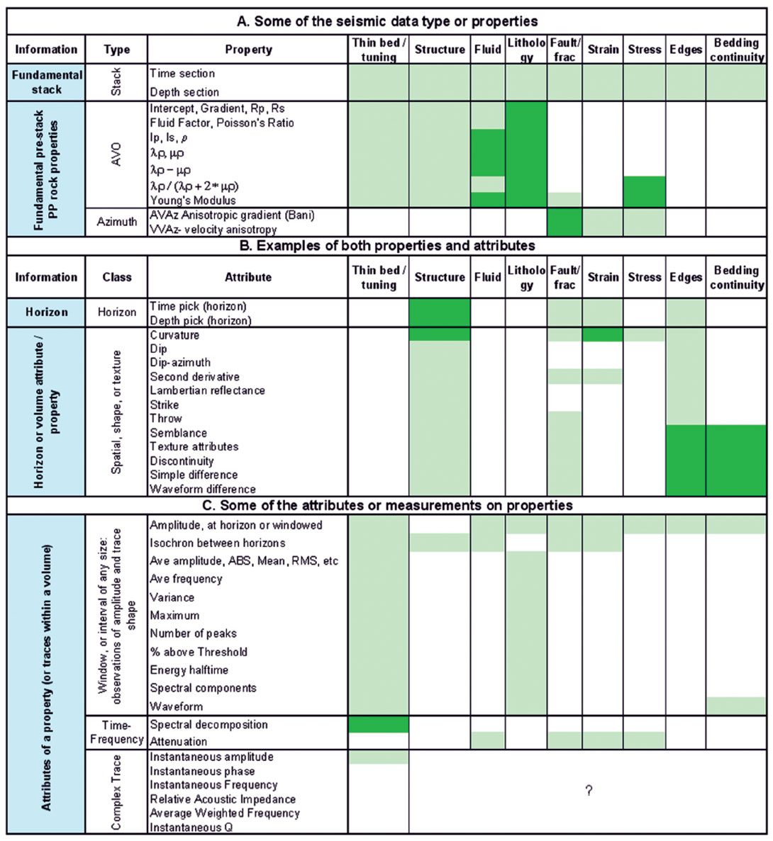
It is difficult to deny Taner’s simple definition, especially given he is the creator of a major set of attributes called the complex trace attributes (Taner et al, 1979). As such, there are literally hundreds of attributes. We propose a modification on how we think of attributes and the interpretive method. The attributes simply form the way in which we extract a measurement from the data. Although there are many attributes, and arguably a near infinite way of extracting or creating them from data, the definition and creation of attributes are not currently our most important focus. We need to consider the physics of our problem first and foremost. It may serve us better to divide this aspect of the interpretive problem into two parts:

1. Seismic properties, which are the major types of information or data contained in the seismic experiment.
2. Seismic attributes, which are the particular measurements of the properties.

We will not generally know at the beginning of a new project which attribute we will use, for it is true that the exact measurement method is largely data dependent. We will be much better off considering instead which seismic property has the best chance of solving our physical problem. Our primary early goal must be towards choosing the best seismic properties. The attributes can follow. The details of the data still have a part to play, but this is typically a matter of parameters like windowing or accounting for tuning effects.

Table I illustrates this new way of thinking about seismic attributes and properties. The table is illustrative rather than exhaustive. Some of the major seismic properties are listed in the first part of the table. These data types are the key things to think about early in a project. The attributes that subsequently follow are extracted on these properties. Some measures have elements of both, such as curvature, which can be measured from another property volume, but may itself be argued as a property due to its relationship to strain. Chopra and Marfurt (2007b) have devoted an entire book describing these special measures. This table, or rather the notions behind it, allow us to formulate our general method of quantitative interpretation.

The key elements of quantitative interpretation

There are many ways that quantitative interpretation may be performed, but there are common elements to most of those methods. The key components include:

1. Identify the earth properties of interest. This is the question that needs to be answered, and is often crafted from an understanding of cross-discipline technical business needs.
2. Identify the seismic data type (properties) that have the most unique relationship to the earth properties of interest. This is the general theoretical relationship. For example, certain AVO inversion volumes may be determined to have the most unique relationship to a question of lithology in a given problem. List the assumptions and limitations in the theoretic relationship.
3. Process the seismic data with a strategy to produce the best quality data possible. This includes performing elastic inversion, azimuthal inversion, curvature, or whatever other work is required to produce the data attributes or volumes most relevant to (or with the greatest uniqueness to) the theoretical relationships of interest.
4. Identify and accumulate control data for calibration, verification, and uncertainty analysis. This may include well log data, core analysis, fracture stimulation data, or production data.
5. Identify the best attributes of the seismic properties. This is done by empirical calibration of various measurements of the seismic property data to the control data. This is both data dependent and theory dependent. The process is quantitative and produces a specific, empirical relationship between seismic data and the earth property of interest. The formulae produced from this work must be consistent with theoretical expectation. In the absence of actual well ties, careful forward modeling may be used to estimate the local quantitative relationship. This may sometimes also be employed in addition to the control data. Multi-attribute predictions, neural network approaches and cross-plotting may also be employed here.
6. Produce the raw seismic attribute maps and measurements using the local optimized windowing methods from #5.
7. Apply the transformation to the seismic attributes to create the quantitative map, volume, or section, of the earth property of interest. Note the transformation formulae of the map.
8. Measure the quality of the prediction against any and all control data. Correlation coefficients or other measures of correlation, and tests for statistical significance should be performed whenever possible. Sources of error should be listed, and measures of uncertainty should be calculated wherever possible.

Correlating data: making different data types talk

In order to perform quantitative interpretation, the seismic data must be compared or correlated with the geologic or engineering data. These comparisons may have to be made between numerous seismic attributes, and in numerous ways. Both the seismic data and the geologic or engineering data must be measured and conditioned in order for the comparison to work. The type of well control may be critical: vertical wells and horizontal wells have different strengths and limitations in comparison to seismic data. The data conditioning of either type of well data or the seismic data has both practical and theoretical elements. Changes in data support (or size) are often important (Isaaks and Mohan, 1989) as seismic data is typically much more coarsely sampled vertically and laterally than well data. This relationship is sometimes reversed with engineering data such as closure stress measurements, which may sample earth properties many seismic bins in size.

All methods of comparison require the seismic data values to be somehow gridded in x,y,z space with the engineering or geological control data mapped to the same bins. Hunt et al (2008) represented Viking Phi-H values from vertical wells as tops that were subsequently co-located with binned seismic AVO reflectivity values. This made sense because the Viking reservoir was thinner than a quarter wavelength, making reflectivity seismic measures naturally comparable. The small scale bulk geologic property of Phi-h was also much more natural to use than, for instance: maximum porosity, average porosity, or thickness of the interval. The bulk property of porosity times thickness accounted best for tuning, thickness, and quality. This property effectively handled the support issue between the data kinds. Phi-h is also meaningful economically as an indicator of reserves and potentially even performance. Treating such a measure as a top at an assigned time or depth is a simple and effective way of comparing these data types.

Horizontal well log data can also be treated as a top, but the handling is not as natural. Hunt et al (2010a) illustrated this in their comparison of horizontal well image log fracture density data with surface seismic fracture predicting properties. In this work, the horizontal well data were up scaled into bins that were then assigned to pseudo vertical wells and tops at the correct x,y,z locations. The top value corresponded to the up scaled fracture density from the image log. The up scaling proved to be challenging to the authors, who performed it in several steps. The work was perfectly valid, but was laborious due to the unnatural step of treating horizontal data as a series of vertical wells.

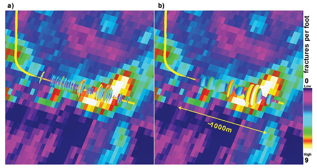
It is more natural and practical to develop software solutions that allow horizontal well log data to be compared to seismic data directly. Schultz et al (1994) and Hampson et al (2001) recommended performing attribute comparisons to vertical well logs rather than tops. Although horizontal drilling is now ubiquitous in resource plays, software solutions allowing such comparisons of horizontal logs and seismic data have only recently been developed. Hunt et al (2011) demonstrated this with the same data that had previously been treated as tops. Figure 1 depicts this handling of horizontal image log data and surface seismic data. Up scaling of the image log data is essential and can either be carried out in the software itself, or prior to loading the log curves into the software.

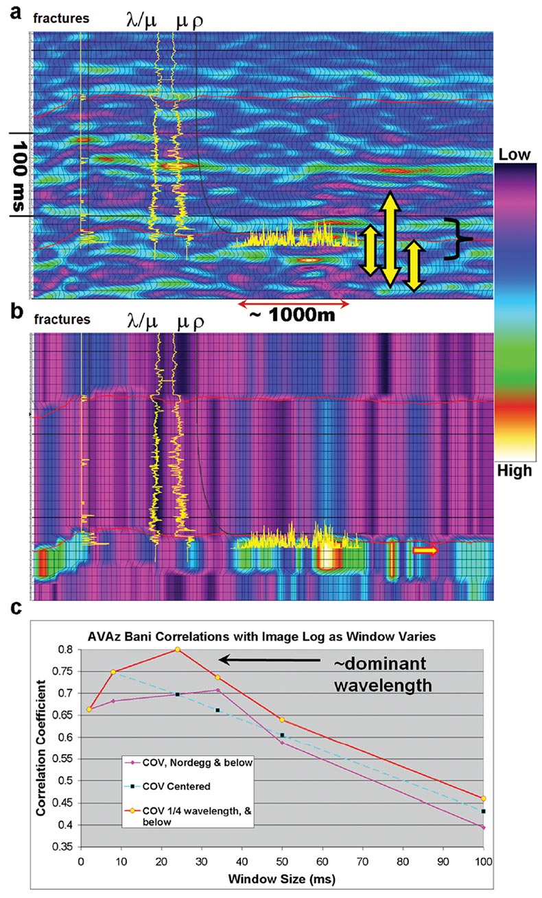
The attribute extraction method may also be important, and may vary depending on the nature of the seismic property being considered. For instance, Hunt et al (2011) showed that layer properties such as VVAz could be tied to image log data in a very straight forward fashion because the property is invariant within the layer. As such, any measurement within the layer yields the same information. This was contrasted against AVAz data, which is an interface property and therefore subject to tuning. Figure 2 illustrates these differences for the Nordegg zone. In the figure, image log data is shown for both a vertical and a horizontal well. Figure 2 (a) shows the AVAz Bani attribute is extracted with root mean square (RMS) averaging over three different window types of various lengths. The windows are described relative to the Nordegg horizon pick. Figure 2 (b) illustrates the VVAz velocity anisotropy attribute is extracted by any pick within the Nordegg interval. Figure 2 (c) shows the correlation coefficients for the AVAz anisotropic gradient (Bani) attribute and the horizontal well image log depending on the window size and position relative to the Nordegg horizon. The best correlations were produced from the window that started 1/4 of a wavelength above the Nordegg and ending 3/4 of a wavelength below the Nordegg top. The AVAz attribute is higher resolution than the VVAz attribute, which is limited by the smallest layer from which azimuthal velocity variations can be accurately picked. Smaller AVAz windows might be expected to work best, however noise in the solution can be a factor. This means that in practice, there may be a trade-off between noise handling with larger windowing and discrimination of the precise interface with smaller windowing. The optimal windowing for AVAz is likely to be data dependent, and most sensitive to tuning, wavelet size, similarity of rock type, and noise.

Time versus depth and the special case of engineering or geomechanical data

The seismic data attributes being correlated can tie the log data in a variety of ways, depending on the software. In some cases, an attribute can be gridded, and the x,y grid can be correlated to the up scaled log data, which is located within the x,y grid. This case would have tremendous flexibility in terms of how the seismic property was measured, and does not require the vertical time or depth (z) dimension to be explicitly addressed. Virtually any attribute with any window could be extracted and located with the well data with this method. In other cases, it is more appropriate for the seismic-to-well tie to truly take place in x,y,z space. For this to happen, all the data types must be represented in either the time dimension or the depth dimension. For the purposes of correlation, it does not matter if the seismic data is represented in depth to tie the well data or if the well data is represented in time to tie the seismic data. Either approach requires that some or all of the data undergo a transformation to the same vertical dimension, and undergo some sort of tying or shifting procedure. Microseismic to surface seismic data requires the same considerations, but again as far as correlation goes, there is no advantage to either the time domain or the depth domain. The choice of domain is a practical matter that is dependent on the software and perhaps on other elements of the data handling strategy or ultimate goals of the work.

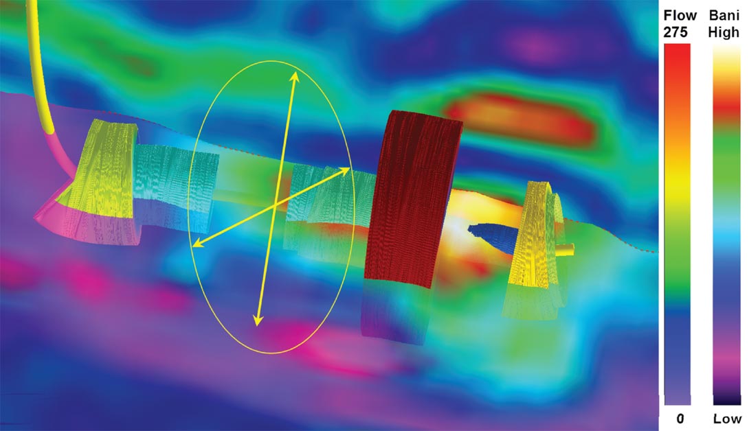
Some kinds of engineering or performance data require more consideration regarding support and how to tie data. For example, how should fracture stimulation data or production test data in a multi-stage fracture treated horizontal well be handled? Both the fracture stimulation and the production data are dependent not only on the earth properties directly coincident with the completion and production interval, but also to an area of influence about that position (Economides and Nolte, 2000). In such a case, the seismic data may have to be weighted by this area of influence and gathered prior to correlation with the engineering data. Figure 3 illustrates a horizontal well with interval flow rate data. Seismic property data that might be compared to this flow rate log could be gathered and binned in a variety of ways. Some software allows the user to define a cylinder of defined x,y,z size about the wellbore, and to accumulate seismic property data into attributes within the cylinder. The yellow arrows illustrate the idea of defining an area about the well bore to accumulate property data for comparison. Distance weighting would be desirable in such a scheme, especially if the user were able to parameterize the weighting by modeled area of influence data from fracture stimulation models.

Simpler methods involve a simple seismic bin to log mapping, all of these methods involve notions of support and influence implicitly or explicitly.

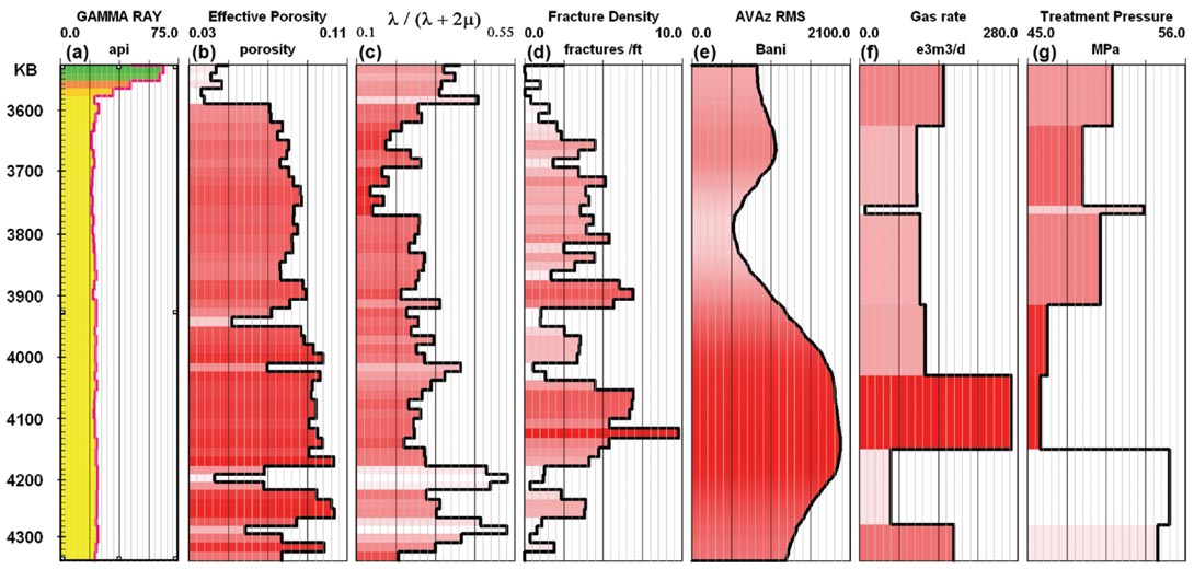
The extracted seismic data can then be compared in cross plots or in log-view with any of the log or engineering performance data. Figure 4 illustrates some of the support issues involving engineering, well log, and seismic data. The figure combines log data such as gamma ray, petrophysically derived effective porosity, bound Poisson’s ratio (Goodway et al, 2010), and image log fracture density with seismic AVAz anisotropic gradient, and with fracture treatment interval data such as average treatment pressure and production log interval flow rate data. There are correlations between many of these data types, although each of these data types have different support, or bin sizes. Even with the log data up scaled to 15m bins as in Figure 4, there are gross differences in support between these data. It is possible to correlate these data as they are, but not desirable to do so, until the differences in support are handled correctly. Isaaks and Mohan (1989) describe some methods for up scaling. This example has particularly egregious support issues because the seismic AVAz attribute comes from 5 by 3 binned gathers, which changes the true support of the data, and because the completion intervals are many seismic bins in size. In some more recent drilling, smaller completion intervals are used, which reduces the disparity in support. None of these problems are insurmountable, however they must all be dealt with in order for the comparisons to be as accurate as possible. Some software is logcentric, some software uses the seismic bin as the reference for support and data to data mapping, and some software uses the completion interval as the reference for support and or data to data binning. Any of these methods can be made to work if the support and mapping issues are handled correctly, and the best method is likely data dependent.

Case studies: to be found in Part II, published in the next issue of the RECORDER.

Conclusions

Quantitative interpretation is the numeric estimate of the earth property of interest from geophysical data. We have described the key elements of quantitative interpretation, and demonstrated them in several examples. The method can be used for a variety of purposes, but is being emphasized today in response to its need relative to the pursuit of tight reservoirs and engineering applications.

Quantitative methods are neither new nor unnatural; these objective predictions are the reason we invest in geophysical data in the first place. The method is limited by the strength of the theoretical relationship between data and predicted earth property, by the quality of the data, and the certainty of the local calibration. Quantitative methods are best applied with consideration of physics rather than a rush to data mine. We have shown that choosing the best seismic measurements should first be concerned with finding the most physically relevant seismic properties prior to the pursuit of the most optimal attributes of those properties. In no sense does quantitative interpretation remove the problems of non-uniqueness, or eliminate uncertainty, or remove noise. The method does not necessarily increase accuracy. It may, however, provide an estimate of what the predictive accuracy is. Misapplied, quantitative interpretation can lead to overconfidence. This being said, careful application of this philosophy should give the practising geophysicist a better chance of identifying the best processing flow, the best local attribute, the approximate level of predictive accuracy, and most importantly produces a measurable set of useful predictions.

There are two sins in decision making: rushing to conclusions, and failing to make a conclusion. Quantitative methods must be pursued thoughtfully, with careful reference to physical theory, and with strict discipline in order to minimize the first mistake. Avoiding the second mistake is implicit to the method. Making an estimate or conclusion is not something we can avoid doing if we are to be of any use to the business challenges of today and tomorrow. Some may claim that the “old ways” work just fine, so why should we emphasize these new, arrogant, quantitative methods? This is a false argument. Concluding our work with a time structure map or an amplitude map instead of a depth estimate or an estimate of Phi-H does not avoid arrogance, it only minimizes usefulness. We are here to make estimates, so let us make them as well as we can.

Acknowledgements

We would like to thank Fairborne Energy Ltd for permission to show this work, and CGGVeritas Multi-Client Canada for permission to show data licensed to them. We would also like to thank Nicholas Ayre, Emil Kothari, Alicia Veronesi, Alice Chapman, Dave Wilkinson, Dave Gray, Darren Betker, and Earl Heather for their work on this project, and Satinder Chopra for his advice.