Traveltime and amplitude based techniques to detect seismic anisotropy have inherent differences in their assumptions and the underlying physics used to describe the seismic response. For this reason, they often produce conflicting solutions, which can lead to inconsistencies between the results. Traveltime methods estimate an interval property, providing an easy to interpret result regarding the anisotropic medium. Amplitude methods estimate an interface property, and in conjunction with its simplifying assumptions such as an isotropic overburden or invariant symmetry axis azimuth, can lead to complications in its interpretation. To address these issues, we implement an azimuthal amplitude-variation-with-offset inversion to estimate the fast and slow shear wave velocities. This produces a layer-based measure of anisotropy that is easier to interpret. This workflow was validated through a case study over a tight siltstone reservoir in British Columbia, Canada, aimed at investigating the presence of fracturing in the reservoir zone. The results of the azimuthal amplitude inversion identified areas of increased anisotropy that were consistent with large-scale structural changes, providing a more quantitative measure of anisotropy from which the presence of fractures can be inferred.
Introduction
Conventional techniques to detect seismic anisotropy can be categorized as traveltime or amplitude based methods, commonly known as velocity variation with azimuth (VVAZ) and amplitude variation with azimuth (AVAZ), respectively. Both these methodologies exploit the anisotropic character of the medium but detect different manifestations of the anisotropic seismic response, where these differences often lead to ambiguities in their interpretation.
VVAZ techniques make use of traveltime variations in the arrival of seismic reflection events as a function of azimuth. These traveltime variations are the result of wave propagation through anisotropic media, therefore an azimuthal velocity difference corresponding to some chosen interval can be obtained through velocity analysis. VVAZ techniques therefore yield a measure of anisotropy that is an interval property and provide an easy to interpret result regarding the anisotropic medium. AVAZ techniques make use of the changes in reflection amplitudes as a function of azimuth to estimate some measure of anisotropy based on the Ruger equation (Ruger, 1998). Because the analysis is performed on reflection amplitudes, AVAZ techniques yield an interface property. Moreover, assumptions implicit in Ruger style AVAZ techniques such as an isotropic overburden or an invariant symmetry axis azimuth above and below the reflecting interface cause further complications in the interpretation of the results.
Both VVAZ and AVAZ techniques measure some degree of seismic anisotropy but have inherent differences in their assumptions and the underlying physics used to describe the seismic response. This results in the differences often seen in conventional VVAZ and AVAZ products (e.g. Delbecq et al., 2013 and Perz et al., 2013), despite the fact that they should represent the same anisotropic medium. The cause of the anisotropy can be due to a variety of reasons including the presence of fractures or differential stress fields. Whatever the cause, the anisotropy is an inherent property of the medium itself and not the interface. Therefore, amplitude base methods must estimate an interval property to properly characterize the anisotropic medium and to provide consistency with VVAZ results.
In this study, we address the limitations associated with conventional AVAZ techniques by estimating fast and slow shear wave velocities via an azimuthal amplitude-variation-with-offset (AVO) inversion. Subsequently, the ratio of the fast and slow shear wave velocities was computed to obtain a measure of anisotropy.
Data conditioning
As input for the inversion, we generate a series of azimuthally sectored angle-stacks from 5D interpolated pre-stack migrated gathers. Figure 1 shows a polar plot of the relative fold distribution for the data as a function of offset and azimuth. The plot reveals an even distribution of azimuths that range from 0-180 degrees with lower fold at the near and far offsets.
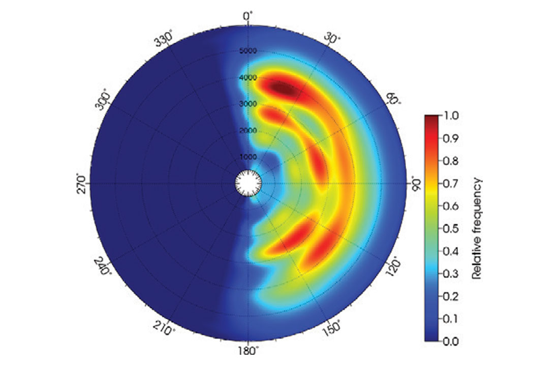
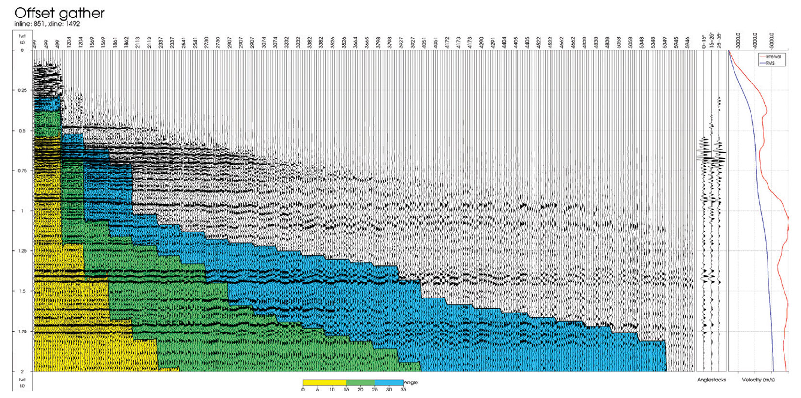
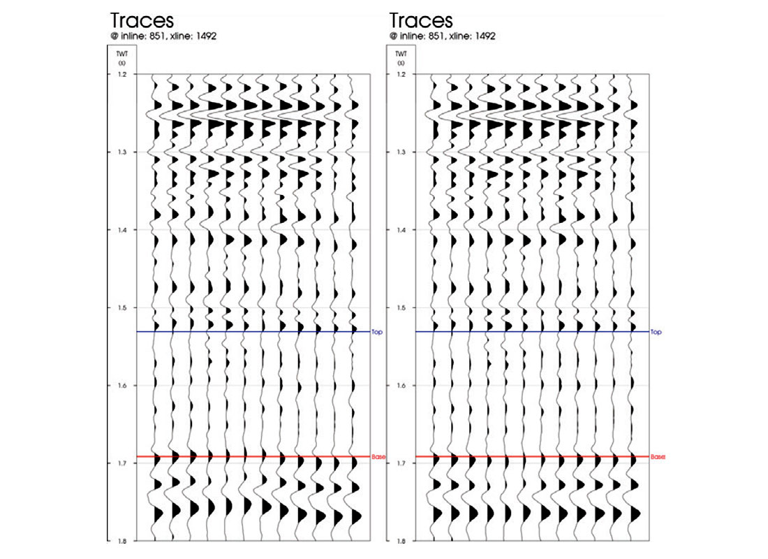
Figure 2 shows an azimuthally sorted offset gather with an angle overlay, the corresponding angle-stacks and velocity functions used to compute the angles. The steps seen in the angle bands are due to the regularly sampled offsets in the interpolation. At the longer offsets, a clear sinusoidal pattern is seen. This is due to traveltime variations from wave propagation through anisotropic media. Prior to inversion, these traveltime variations must be corrected so that the proper reflectivity response can be analyzed. Here, we implement a dynamic time warping algorithm to correct for the residual moveout due to both the kinematic effects of anisotropy and any improper velocity modeling or migration. The warping algorithm computes and applies a smoothly varying displacement field to optimize the cross-correlation between the seismic stacks. Figure 3 shows the effect of warping on a far anglestack sorted by azimuth where the improvement in event alignment can be seen especially at the Base horizon.
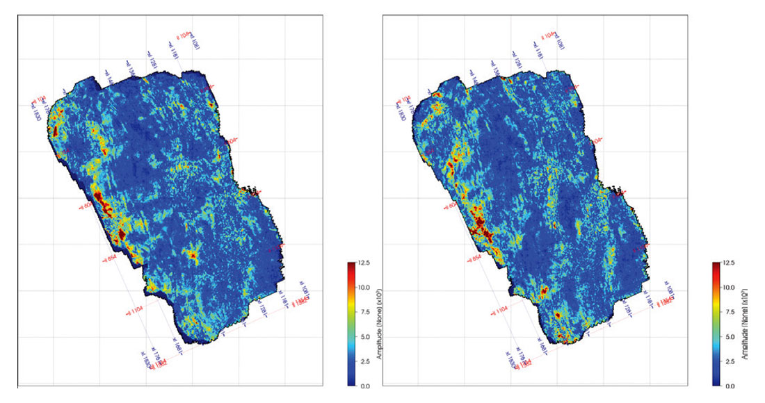
As the azimuthal variations in the seismic response are zero at normal incidence and increase with larger reflection angles, we chose a set of azimuthal angle-stacks such that the number of azimuth sectors increases with increasing incidence angle. This also helps to improve the signal-to-noise ratio for the near angle stack as fold is typically lower at smaller offsets as can be seen in Figure 1. The resulting set of angles and azimuths chosen as input for the azimuthal AVO inversion are shown in Table 1. Figure 4 shows an RMS amplitude map of the far angle-stack at azimuth angles of 15 and 105 degrees, where differences in the reflection amplitudes are evident in specific areas of the survey.
| Stack | Angle (degrees) | Azimuth (degrees) |
|---|---|---|
| Table 1. List of input azimuthal angle-stacks used in the inversion. | ||
| a0z0 | 0-15 | 0 |
| a1z0 | 15-27 | 22.5 |
| a1z1 | 15-27 | 67.5 |
| a1z2 | 15-27 | 112.5 |
| a1z3 | 15-27 | 157.5 |
| a2z0 | 25-35 | 15 |
| a2z1 | 25-35 | 45 |
| a2z2 | 25-35 | 75 |
| a2z3 | 25-35 | 105 |
| a2z4 | 25-35 | 135 |
| a2z5 | 25-35 | 165 |
Azimuthal AVO inversion
The azimuthal AVO inversion used in this study is based on the Psenick and Martin’s formulation (2001) of the reflection coefficient for weakly but arbitrarily anisotropic media. In our implementation, the reflection coefficient is parameterized in terms of the P-impedance, fast and slow shear wave velocities and orientation, fast and slow horizontal P-wave velocities and orientation, and density.
To investigate the reliability of each inversion parameter, we performed a sensitivity analysis using an eigenvalue approach. By constructing a matrix of coefficients corresponding to the reflectivity equation, we compute the eigenvalues to determine the sensitivity with respect to each parameter. It was found that the horizontal P-wave velocity terms have a sensitivity that was less than 1% compared to that of the P-impedance, whereas the shear wave velocity terms have a sensitivity that was on the order of 16% compared to that of the P-impedance. This suggests that the horizontal P-wave velocities cannot be estimated with a reasonable degree of certainty, and as a consequence were excluded from the analysis.
Results and discussion
Figure 5 shows a QC of the inversion results for the P-impedance and fast and slow Vp/Vs. The left panels show the inverted trace in blue and the measured well logs in red. The right panels show variable density displays of the inversion results with log inserts. To obtain a measure of anisotropy, we compute the ratio of the fast and slow shear wave velocities. Figure 6 shows the inverted fast and slow shear wave velocity ratio at a well location with a measured cross-dipole shear wave sonic. Above the Top horizon, the well log measurements and the inversion results show a good match, and the observed anisotropy is up to around 6%. Below the Top horizon, the inversion produces a result that indicates a larger degree of anisotropy relative to the well log measurements. A potential explanation could be associated with the measurement scale of the seismic versus borehole logging frequencies. If fractures are the cause of the observed anisotropy, the difference between the inversion and well log results could be due to a fracture spacing that is much smaller than the seismic wavelength but large compared to the measurement scale of the logging frequencies.
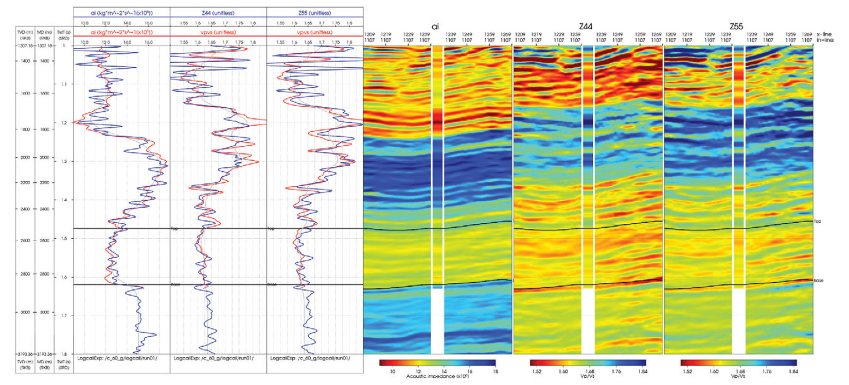
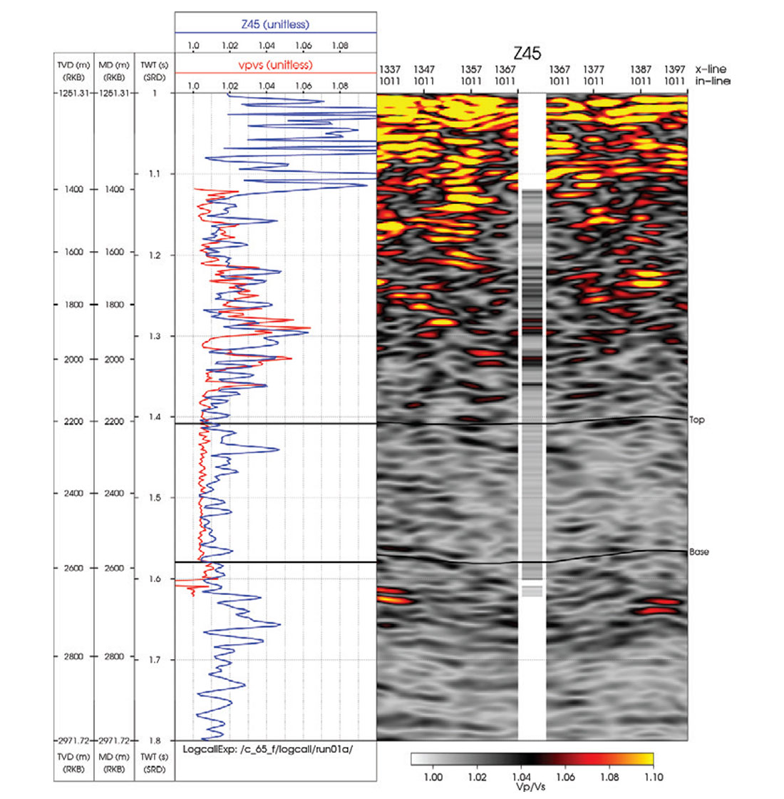
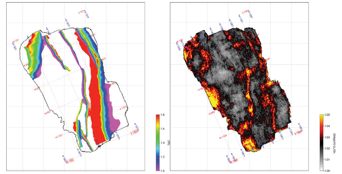
Figure 7 shows the fault interpretation (left) and a horizon slice of the fast and slow shear wave velocity ratio (right) over the reservoir zone. The high anisotropy areas are very much correlated to areas of increased deformation in the fault vicinity. From a structural geology standpoint, areas with large structural variations are more likely to be fractured due to increased deformation or strain. This interpretation however, is indirect and more qualitative, where the degree of anisotropy cannot be quantified. The results from the azimuthal AVO inversion provide supplementary information to the structural interpretation, where a direct measure of anisotropy is obtained, providing a more quantitative interpretation from which the presence of fractures can be inferred.
Conclusions
Discrepancies between conventional VVAZ and AVAZ results often lead to inconsistencies in their interpretation. This is the result of VVAZ methods estimating an interval property versus AVAZ methods, which estimate an interface property. In this study, we estimate the fast and slow shear wave velocities from an azimuthal AVO inversion to provide a more interpretable result regarding the anisotropic state of the subsurface. We demonstrate the usefulness through a case study in a tight siltstone reservoir in British Columbia, Canada, where the objective was to identify areas with greater fracture intensity. The results of the azimuthal AVO inversion revealed areas with an increase in anisotropy, which is corroborated by the structural interpretation to increase confidence and produce a more quantitative result from which the presence of fractures can be inferred.

Acknowledgements
We would like to thank Progress Energy and Sasol Canada Exploration and Production Limited for permission to publish the results of this study, Seitel for permission to show the data and Evan Mutual for his contributions to this project. Klaus Bolding Rasmussen is acknowledged for the development of the inversion algorithm used in this study.


Join the Conversation
Interested in starting, or contributing to a conversation about an article or issue of the RECORDER? Join our CSEG LinkedIn Group.
Share This Article