Introduction
Rulison Field, Piceance Basin, Colorado was approved for development drilling to 10-acre spacing in 2003. The down spacing and hydraulic fracturing within this unconventional reservoir has increased its production five fold in less than a decade. A significant portion of the gas production is from low permeability fluvial discontinuous sandstones within the Williams Fork Formation of the Mesaverde Group. The gas is generated in the thick thermally mature coals of the Cameo Coal interval within the lower part of the Williams Fork Formation and migrates through the natural fractures that connect the reservoir and the coal interval. Development of this reservoir section is a challenge because the sandstone reservoir bodies are thin, generally below resolution of conventional compressional-wave (P-wave) seismic data, and lack acoustic impedance contrast with the surrounding shales. However, these sandstone bodies have a shear-wave impedance contrast with the encasing shale and that is what potentially makes shear waves attractive for imaging of these productive sand bodies.
To test the value of shear waves in imaging tight gas sands we conducted a 3-D VSP survey in Rulison and applied anisotropic Kirchhoff 3-D prestack depth migration to the data. A geologically-constrained migration-velocity model was created by integrating the results from the virtual source method, well logs, interval velocity derived from surface seismic and the Dix-differentiation of the fast (S‖) and slow (S┴) shear-wave NMO ellipses. The resulting common image gathers (CIG) are flat, indicating that the reflection events can be stacked reliably. Moreover the productive sand bodies have been reliably imaged with this technique.
A Brief Background of Shear-wave Tight-gas Sand Exploration
In spite of its abundance, natural gas in Rulison Field is difficult to extract economically. P-wave (compressional wave) surface seismic imaging of reservoir units is impossible. Also, fracture detection within the sandstone intervals from Pwave data is not feasible. While none of the wells in Rulison Field are dry the potential for these wells to become uneconomic exists as gas prices fall below $5/mcf. As the reservoir has not been imaged adequately with conventional seismic methods operator drill wells at a spacing interval that allows them to adequately drain the reservoir (a 10-acre spacing in Rulison). The sandstone intervals in the drilled wells are identified from lithology indicator logs, eg. Gamma ray (GR) logs, and the sandstone intervals are hydraulically fractured.
A limited number of case studies have been published on imaging formations with low P-impedance contrast. The VSP shear-wave imaging case studies have mostly been done in low acoustic impedance contrast formations using P-S data (Nazar & Lawton, 1993; Roche et al., 2005; MacLeod et al. 1999; Macrides & Kelamis, 2000; VanDok & Gaiser, 2001; Rampton (1995); Michelena et al. (2001)). Hokstad et al. (1998) used reverse-time migration on the signatures recorded by horizontal geophones in a walkaway VSP survey in an offshore environment and found that the shear-wave migration was noisy (because of limited available migration aperture) yet with better resolution (attributed to short wavelength of shear waves in their study). A case study with PS VSP imaging, particularly for tight sand detection has been documented by O’Brien & Harris (2006). They succeeded in using walkaway VSP data to image the sandstone bodies in the low porosity Bossier and Cotton Valley sands in East Texas Basin. They did 2-D imaging and concluded that PS waves are sufficient to image the sandstones in their area of study. To the best of our knowledge, a 3-D non-converted shear-wave VSP depth imaging case study of tight gas sands is neither available in literature nor reported in industry. In this paper we would use shear-wave sourced VSP shot records to detect the elusive sandstones.
VSP Data Acquisition at Rulison
The Reservoir Characterization Project at Colorado School of Mines acquired a 3-D, multi-component VSP survey in 2006.
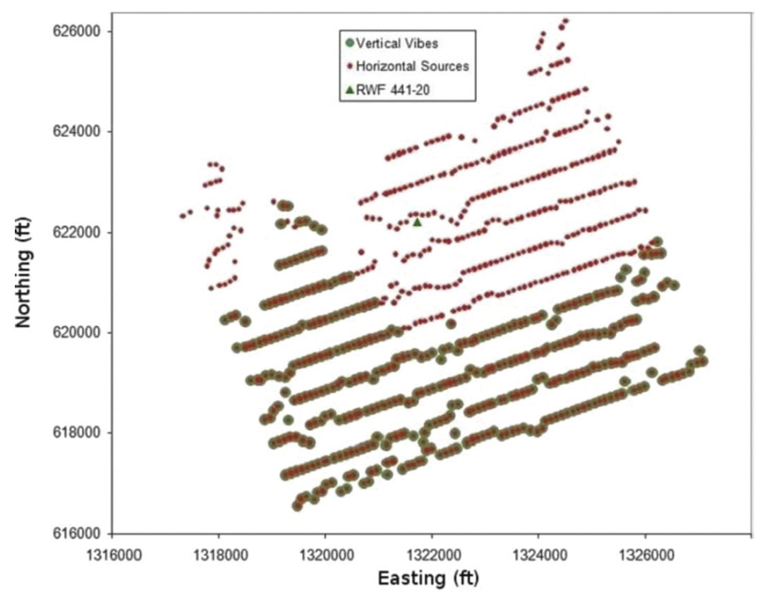
The VSP survey was a part of a project for integrated characterization and monitoring of Rulison field using surface seismic, VSP, geomechanics, well logs and production data. Two horizontal vibrator trucks were used as seismic sources that generated two mutually orthogonal horizontal ground motions at each of the 700 shots points. One horizontal vibrator was oriented at N70E direction and the other horizontal vibrator was oriented at N20W direction. In addition, a vertical vibrator was operated at about 300 far-offset shot points. The surface locations of the horizontal and vertical vibrators are shown in Figure 1. The 3C geophones (one vertical and two horizontal) occupied 60 levels in the borehole.
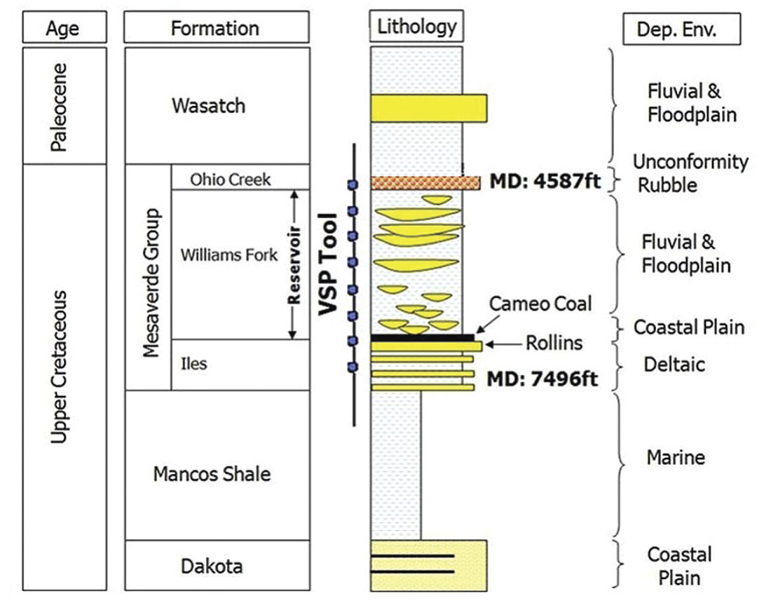
The shallowest 3C receiver is located at the top of the Williams Fork Formation (at 4587 ft) and the deepest receiver is within the Cameo Coal (at 7496 ft) as shown in Figure 2. The receiver spacing in the array is 50 ft. Table 1 details the source parameters in the Rulison VSP survey in 2006.
| Parameters | Vertical Vibrator | Horizontal Vibrator |
|---|---|---|
| Table 1. Source and receiver parameters. | ||
| Model | AHV-4 | M18 (Mertz) |
| Number of Vibes | 1 | 1 |
| Start Frequency | 6 Hz | 5 Hz |
| End Frequency | 120 Hz | 50 Hz |
| Start Taper | 300 ms | 300 ms |
| End Taper | 300 ms | 300 ms |
| Sweep Type | Linear | Linear |
| Listen Time | 5 s | 6 s |
| Sweep Length | 10 s | 10 s |
| Number of sweeps | 6 | 6 |
| Sample Rate | 2 ms | 2 ms |
| Source Points | 300 | 700 |
Shear Wave VSP Imaging of Sandstones
Subsurface imaging is done using a migration procedure that takes seismic wavefields recorded either on the surface or in a borehole as input and computes the location and reflection strength of subsurface interfaces. There are various ways to migrate the input seismic wavefield. A popular method, Kirchhoff migration, is used in this study. Next we describe the fundamental steps we used in this study to image the subsurface using non-converted shear wave VSP data. These steps include-
- Anisotropic velocity model building (for migration), and
- Computation of traveltime and Prestack Kirchhoff depth migration.
In Rulison Field, gas production comes mainly from sandstone beds that are fractured. Shear waves travelling through fractured sandstones split into fast and slow modes. The fast shear wave is polarized parallel to the fracture plane and the slow shear wave is polarized perpendicular to the fracture plane. The procedure to separate the shear waves for all the acquired shots is discussed in Mazumdar and Davis, 2009. In this section, we would discuss how to use the transmitted split shear waves for anisotropy parameter estimation and build an approximate velocity macromodel needed for depth migration of the reflected split shear waves. Next, we migrate the shear wave VSP dataset using the macro-velocity model to recover the image of the subsurface. The interpretation of the shear wave images is outside the scope of this paper and shall be discussed in a sequel paper.
The azimuthal variation of normal moveout velocity for nonconverted modes is described by an ellipse in the horizontal plane (Grechka & Tsvankin, 1998). In this study a hyperbolic moveout approximation is used that accurately describes the traveltime variation with offset. The maximum offset to depth ratio in the Rulison VSP dataset is about 1.4 for the shallowest geophone (measured depth = 4587 ft) and about 0.86 for the deepest (measured depth = 7500 ft). All the shot points on the surface were chosen for the purpose of inversion. Finally, the traveltime needs to be described by a Taylor-series expansion for squared traveltime t2(xα2) where xαis the offset of a source point on a survey line at an azimuth of α. The Taylor-series expansion can also breakdown for shear waves in certain anisotropic media where it can lead to cusps on traveltime curves. However, the cusp will occur only if the anisotropy is sufficiently strong (Helbig , 1966; Musgrave, 1970) even in a homogeneous medium. The cusps do not occur in the Rulison dataset because it requires the value of σ(V) be greater than 0.6 and the source-receiver offsets greater than 4.5 kms.
In Rulison Field, both the overburden and the reservoir interval are anisotropic. The overburden as well as the reservoir interval contributes to the shear wave splitting. The reservoir rocks in the Williams Fork Formation splits the incident shear waves due to the presence of natural fractures in the rocks (Matesic, 2007).
We use the following equation (Grechka & Tsvankin, 1999) to estimate the interval NMO ellipse:

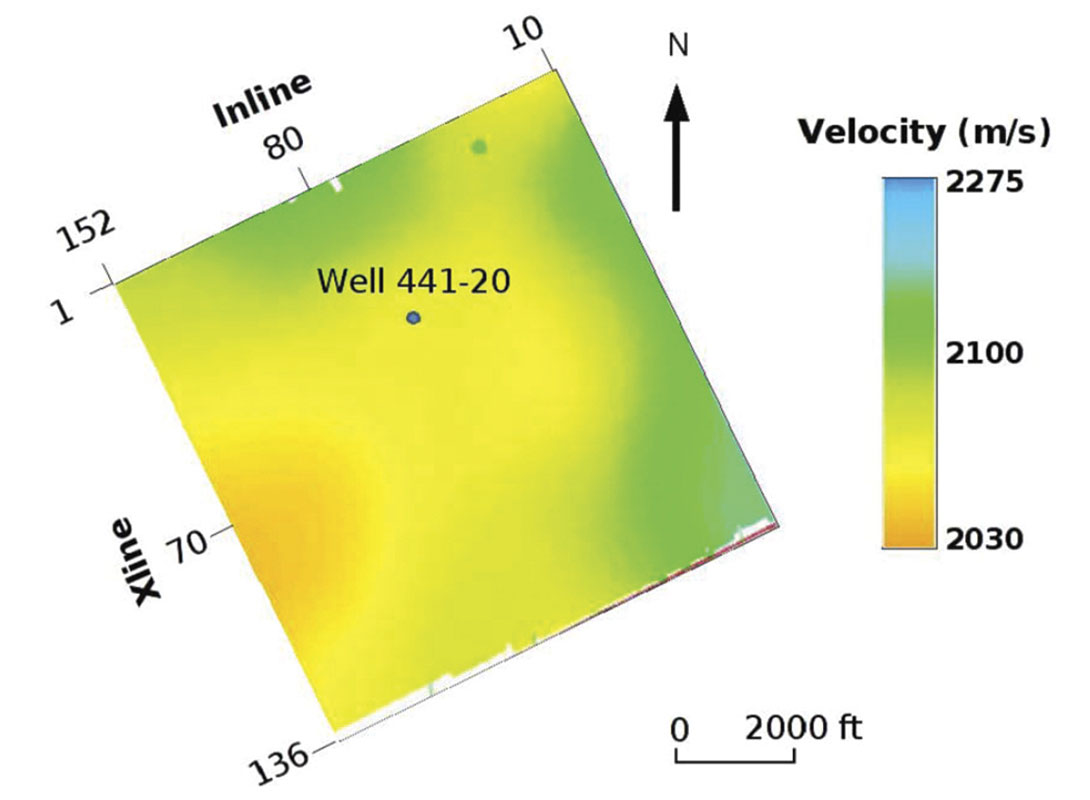
where Wl is the interval ellipse in the l-th layer, W(l) is the effective NMO ellipse in the bottom of the l-th layer, τ(l) is the zerooffset traveltime to the bottom of the l-th layer. In the case of horizontal reflectors it is straightforward to use Dix-type equation 1 to estimate the interval NMO ellipse. Within the RCP survey area, the maximum dip is less than 2 degrees. Thus the dips in the reservoir interval do not affect the azimuthal velocity analysis in the RCP survey area. The azimuthal NMO can also be influenced by lateral velocity variation (Grechka & Tsvankin, 1999). Also, the lateral velocity variation is investigated within the RCP survey area. The dipole sonic logs at various wells in RCP survey area show that the shear wave vertical velocity trend does not vary significantly in the survey region. Moreover, a time slice taken at 2000 ms (within the reservoir interval) shows that there is mild lateral velocity variation. In the RCP survey area we see that the lateral velocity variation is small (see Figure 3). The rate of lateral velocity variation shall be even smaller than the magnitude of lateral velocity variation. Hence, we have not attempted to remove the effect of lateral velocity variation.
The reservoir interval is divided into smaller depth intervals and the inversion is conducted at each layer. For example, the reservoir interval is divided into three pseudo-layers (irrespective of the evidence of any spatially continuous geologic reflector) of 1500 ft each and the Dix-type differentiation is conducted to estimate the interval velocities at each sub-layer. The procedure is repeated with smaller depth intervals, say, three pseudo-layers, each with thickness of 1000 ft. We get comparable results from the Dix-differentiation procedure for both the cases of 3 pseudolayers and 4 pseudo-layers. The interval velocities of fast and slow shear modes are obtained by constructing the matrix Wij for different depth locations of geophones. Then the matrix Wij is inverted and used in equation 1. This gives us the interval Wij-1 (l) which is inverted to get interval Wij for the l-th layer. Finally, the interval NMO velocity ellipses for the fast and slow modes and their orientation can be computed from the coefficients of the inverted matrix, Wij The next section explains how azimuthally dependent NMO velocities can be used for anisotropy parameter estimation in the reservoir section. Because the reservoir rocks are fractured we assume HTI media.
Azimuthal Dependence of NMO Velocity in Reservoir Section
The general NMO equation for a horizontal HTI layer that fully honors the 3D behavior of phase- and group-velocity vectors is described by Tsvankin, 1997. The azimuthal dependence of NMO velocity for a non-converted mode is expressed as:

where α is the angle between the survey line and the symmetry axis, and A is an anisotropic term given by:

Equations 3 to 5 show that the azimuthal dependence (also valid outside the symmetry planes) of NMO velocity for all the three non-converted wave modes can be expressed through Thomsen parameters of the equivalent VTI medium. The NMO velocity contains just three unknowns. We require measurement of NMO velocity on at least three different azimuthal angles (Rüger & Tsvankin, 1997). The resulting NMO velocity can be inverted for the vertical velocity, the axis orientation, and the parameter A for any given pure mode. Here all the shots have been used for estimation of these three Thomsen-style parameters. Also,

The exact NMO velocity in the symmetry-axis plane for the P, S‖ and S┴ modes (Tsvankin, 1997) is given by:
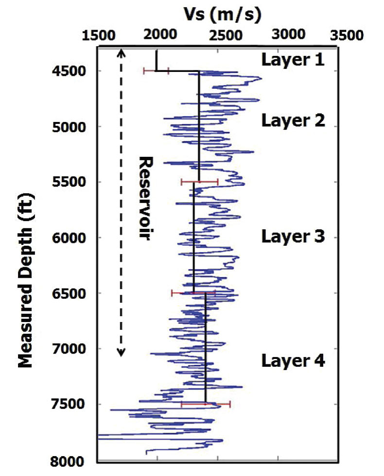
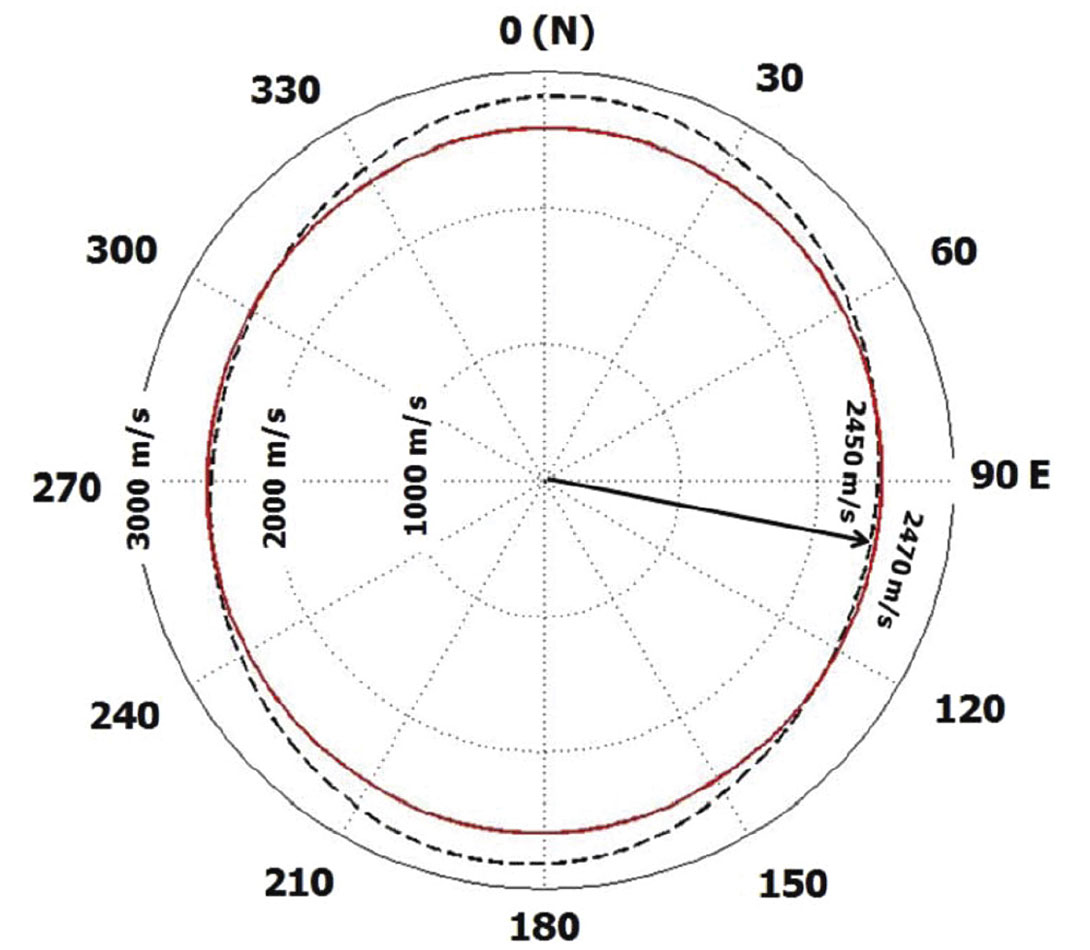
The vertical interval velocity and the anisotropy parameter, A, corresponding to the two shear wave modes is estimated for the overburden and the reservoir interval in Williams Fork Formation. The estimation is based on equations 6 and 7. The vertical interval velocity profile within the reservoir interval for S mode is shown in Figure 4. The error bars (shown in red) are estimated by applying one way time picking error of 1 sample (2ms). The vertical velocity profile for S┴ mode is not shown in Figure 4 because the average splitting coefficient over the reservoir interval is found to be small (1%). The interval NMO ellipse corresponding to pseudo-layer 4 (base of reservoir) is shown in Figure 5.
The values of σ(V), γ(V) and the semi-major axis of the interval NMO ellipse are also estimated for the overburden and the reservoir interval. The overburden has σ(V) = 0.17 ± 0.06 and γ(V) = 0.03 ± 0.02 and the reservoir interval has σ(V) = 0.11 ± 0.07 and γ(V) = 0.015 ± 0.01. Small values of σ(V) and γ(V) suggest that the rocks are unfractured in the reservoir interval of well 441-20. Grechka & Kachanov (2006) indicate that in dry circular cracks we expect approximate elliptical anisotropy (ε(V) ~ δ(V)) leading to σ(V) ~ 0. This is the case in the RCP survey area where we do not have a water leg in the reservoir section of the Williams Fork Formation. However, the overburden above the Williams Fork Formation has water-filled cracks (Yurewicz et al. 2008). In this case we can expect a non-zero value of σ(V). The azimuth of the semi-major axis of the overburden is estimated at 165°- 25° and for the reservoir it is 100°- 40°. The semi-major axis in the reservoir interval does not vary with depth and is consistent with the FMI interpretation of fractures in well 441-20 (Garrow, 2006). There is larger uncertainty of estimating the principal direction in the reservoir interval because of small fracture density at the location where the well 441-20 is drilled. The shear wave splitting from virtual source studies also suggests low fracture density within the reservoir interval. The evidence of low fracture density is also found in the FMI interpretation for fractures in well 441-20 (Garrow, 2006).
Velocity Macro-Model for VSP Migration
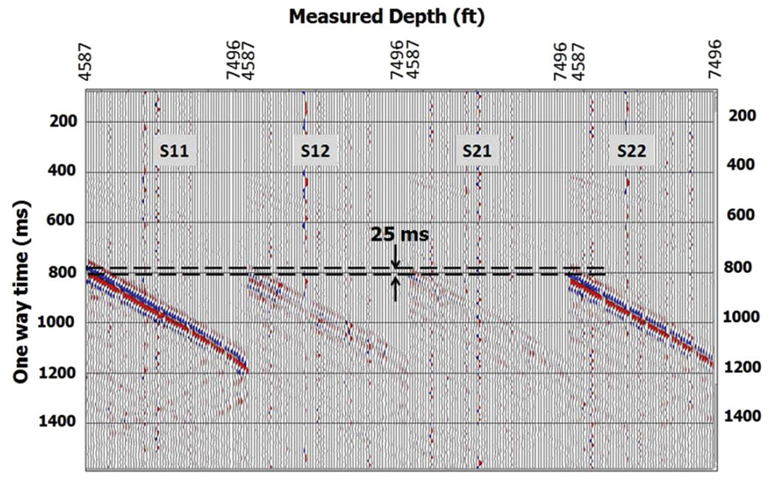
The vertical velocities for the fast and slow shear waves and the anisotropy parameters σ(V) and γ(V)) control the kinematics of these pure modes. It is thus important to take the anisotropy parameters into account when building a migration velocity model for the S‖ and S┴ waves. The simplest model that explains the splitting of shear waves at normal incidence is shown in Figure 6, and can be assumed to be HTI. Examination of a nearoffset (250 ft) VSP shot record shows 25 ms splitting at the shallowest geophone (MD=4587 ft). This amounts to the splitting coefficient, γ(V) = 3% in the overburden. The medium parameters for the overburden are estimated from the NMO ellipse as described above.
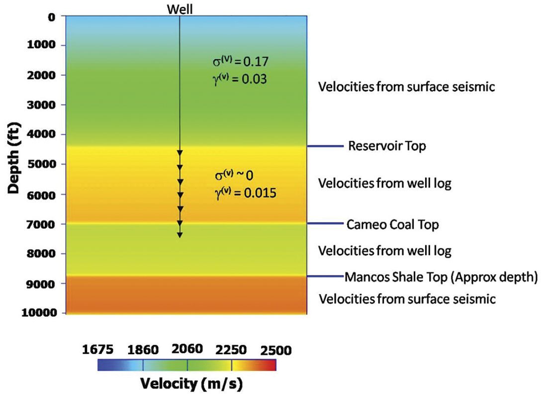
For the reservoir interval we find that the dipole sonic derived shear wave velocity and velocities from Dix-differentiation are same. Choice of either of these velocities can be used to populate the velocity model in the reservoir interval. The anisotropy coefficients σ(V) = 0 and γ(V) = 0.015 are assigned to the reservoir interval of the macro-velocity model. Although small, the anisotropy parameter of the reservoir, γ(V) = 0.015, is crucial in optimal depth-positioning of the reflectors within the reservoir interval. The interval velocity in the coal layer is assigned a constant value of 1900 m/s (derived from well log) and anisotropy coefficients are set to zero. This could be an inappropriate assumption because coal has orthorhombic symmetry. The VSP survey did not have enough geophones to estimate the anisotropy parameters in the coal interval. The well does not penetrate to the Mancos Shale layer (below the Cameo Coal interval). So, it makes sense to populate the interval velocity using the surface seismic derived interval velocity. In Mancos Shale layer σ(V) = 0 and γ(V) = 0 is assumed and hence the velocity model in this layer is also approximate. A 2D line passing through the macro-velocity model is shown in Figure 7. This velocity model shall be used for migration of the VSP shot records.
Kirchhoff Prestack VSP Depth Migration
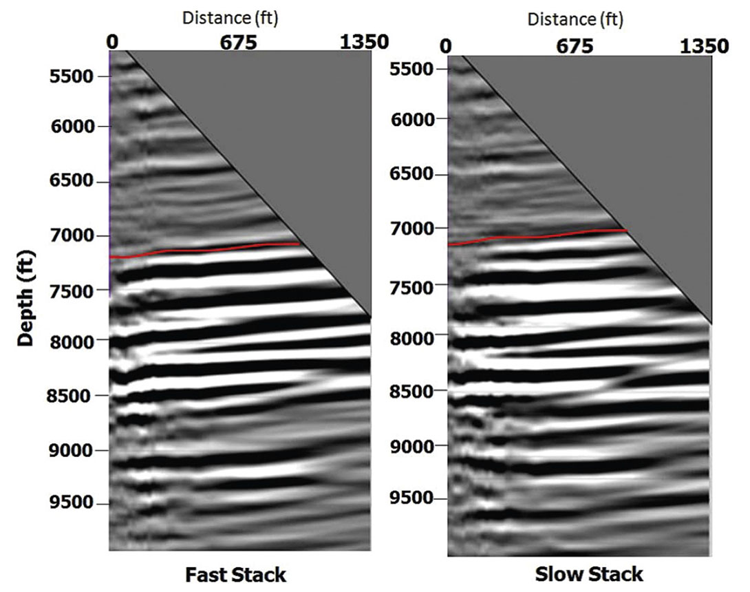
The primary objective of migration in the Rulison VSP survey area is to image the sandstones in the reservoir interval and in the Cameo Coal layers. The Kirchhoff depth migration method is used to migrate the shots in the RCP survey area. The Kirchhoff migration code had only the obliquity factor built into it and hence is not a true-amplitude migration. True-amplitude Kirchhoff migration additionally requires geometrical-spreading factors. This spreading factor is necessary to calculate the weight term for migration. All the shots in the survey were divided into 60 x 3° azimuth sectors. The shots in the individual azimuthal bins were migrated using Kirchhoff migration scheme with migration aperture of 5500 ft. This aperture is considered adequate given the maximum source-receiver offset of 6500 ft. The output grid was in polar coordinates with size of 20 ft x 3° x 10 ft. The grid size is 20ft (in radial direction from the well 441- 20), azimuthal increments of 3° and depth increments of 10ft. An output-grid dimension larger than 20 ft x 3° x 10 ft resulted in spatial aliasing and significant degradation in the migration output. The azimuthal sectoring and migration was independently done for both S‖=> and S┴-wave shot records. The image gathers were stacked resulting in 60 radial depth sections. The migrated stack output in polar coordinates was converted back to rectangular coordinates using bilinear interpolation. Conversion of polar stacks to rectangular coordinates resulted in 135 inline x 135 crossline stacked sections each separated by 20 ft. Producing stack sections in a rectangular coordinate system enables loading the migrated data in commercially available visualization systems (say, Landmark’s SeisWorks, Jason Workbench etc.) for further interpretation. The common image gathers and reflection stacks for both fast and slow modes of shear waves are shown in Figure 8 and Figure 9 respectively.
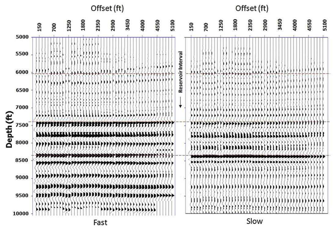
The common image gathers (shown in Figure 4.13) are for both fast and slow shear waves. We observe some image distortions in the depths from 5000 ft to 6000 ft. The distortion, however, disappears at depths exceeding 6500 ft. The reason for the distortion is currently not well understood. It is possible that the distortions are related to inadequate aperture-effects for reflectors close to shallower geophones (4587 ft to 6000 ft) or it could be real and related to a fault. Further evaluation and geologic interpretation of the migrated data shall be made in a sequel paper.
Conclusions
Ray tracing in anisotropic velocity model is required for Kirchhoff depth migration of the shear wave reflections. In general, anisotropy parameters can be estimated by means of migration velocity analysis. However, a plausible velocity model can also be constructed using the interval velocities derived from surface seismic stacking velocities for shear waves, dipole sonic logs and the anisotropy parameters (σ(V) and γ(V)). The values of (σ(V) and γ(V)) in the overburden and reservoir interval are estimated using the traveltime of transmitted shear waves. The overburden has larger values of (σ(V) and γ(V)) than in the reservoir interval at the VSP well location. Reflection events in the common image gathers were found to be flat resulting in a prestack reflection dataset suitable for stacking.

Acknowledgements
The authors thank sponsors of RCP and RPSEA consortium for research funding. Help by Dr.Bruce Mattocks (CGGVeritas) for data processing, Prof. Ilya Tsvankin (CSM) for seismic anisotropy and Dr. Jonathan Liu (ExxonMobil) for 3D migration is also appreciated.
Related Reading


Join the Conversation
Interested in starting, or contributing to a conversation about an article or issue of the RECORDER? Join our CSEG LinkedIn Group.
Share This Article