Shear-wave sourced 3-D VSP Image Interpretation of Tight Gas Sandstones in Rulison Field, Colorado

Introduction

Exploration and development of tight-gas sandstone reservoirs relies heavily on understanding the distribution of sandstone bodies in the subsurface. Shear-wave sourced 3-D vertical seismic profiling (VSP) data are used for sandstone detection and fractured interval delineation. We apply anisotropic Kirchhoff 3-D prestack depth migration to the shear wave VSP reflection data. The depth migrated images tie with the well logs and the surface seismic data. The VSP images show subtle stratigraphic features involving sandstone intervals in the Williams Fork Formation and pinchouts in the coal beds within the Cameo Coal interval. Structural features, especially faults, previously unnoticed on surface seismic data are now clearly visible. At a given depth interval, the differences in reflection amplitudes of split shear waves indicate fractured zones. The shear-wave VSP data can be used as a complementary dataset to other commonly acquired data such as surface seismic, well logs and core data, to improve reservoir characterization.

A Brief Background of Shear-wave Imaging in Rulison

Shear-wave sourced 3-D VSP data was acquired by the Reservoir Characterization Project in Colorado School of Mines in 2006. The high-quality VSP data was processed and migrated using an advanced procedure of pre-stack anisotropic Kirchhoff depth migration. The details of the survey parameters and the depth-migration procedure are discussed in a sequel paper. The seismic events in the entire common image gather (CIGs) after the migration are found to be flat and are stacked to get the image of the subsurface. The remarkable aspect of the shear wave imaging procedure is that we get two images of the subsurface from the given survey. They are the fast and slow shear-wave images. The fast shear wave image gives information of the lithology and the slow shear-wave image provides additional information about the fractures in the rock formation.

In the Rulison survey, surface seismic data was acquired simultaneously with the VSP data. In principle, the same reflected wavefield is recorded by the geophones in the well and at the surface. In this study we shall focus on the interpretation of the recovered VSP images and evaluate the improvement over the existing surface seismic images.

Quality of the VSP Images

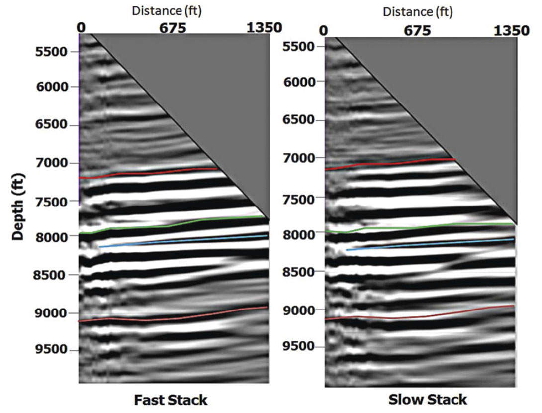
In this section we assess the quality of the recovered fast and slow shear-wave VSP stacks. The quality shall be assessed in terms of the depth positioning of the reflectors. If the migration velocity macro-model (Mazumdar and Davis, 2010) is correct, then VSP migration should position the image of reflectors at the actual depth they exist in the subsurface. Both the fast and slow shear wave VSP stacks should show consistency in depth positioning of their seismic events. Once the VSP images qualify in this depth consistency test then we need to verify whether either of the VSP images ties with the recorded well logs in the VSP well. This VSPwell tie shall facilitate further interpretation of the VSP images and shall be discussed subsequently.

A few prominent continuous horizons are picked on the fast shear wave VSP stack and the same horizons are put on the slow shear wave VSP stack. All these picked horizons belong to the Cameo coal interval (7000 ft) and below. This deeper interval is chosen for depth evaluation because the acquisition parameters in this VSP survey provide sufficient migration aperture in this depth interval. This is also evident from the stack sections as we have no apparent migration related artifacts (such as migration smiles) in them. Four prominent horizons at the well 441-20 location (irrespective of the drilled depth) are chosen and interpreted on the fast shear VSP stack. As shown in Figure 1 they are the red horizon (at 7200 ft measured depth), green (at 8000 ft), blue (depicting a pinchout at 8200 ft) and a brown horizon (at 9150 ft) close to a reflector in Mancos Shale interval. It is observed that the reflectors picked in red, green and blue match reasonably well on both fast and slow shear wave VSP stacks. However, we observe a prominent depth mismatch for the interface at 9150 ft picked in brown color. This is possibly because of poor representation of migration velocities and a lack of available migration aperture in the deeper interval. These deeper layers close to the Mancos Shale are not the focus of the current VSP survey and shall not be discussed further.

VSP images are susceptible to source statics errors. If there is error in the estimation of source statics then this error propagates in the VSP images thus resulting in degradation of image quality. Virtual source 1D reflection seismograms (Mazumdar et.al. 2008) are not affected by the overburden effects and source statics. The kinematics of the virtual source 1D reflection seismograms are correct and are suitable for tying with the VSP image in time domain. Figure 2 shows the tie of slow shear VSP image and virtual source 1D reflection seismogram at the drilled well 441- 20. It shows that the VSP image is not affected with the overburden effects at the well location.

VSP Image Tie with the Well Log

Both the VSP image and the recorded well logs are in the depth domain. Lithology indicator logs like gamma ray (GR) can be tied with the VSP image (say, the fast shear image) through a zero-offset shear wave synthetic seismogram. The tie is shown in Figure 3.

The zero offset shear wave synthetic seismogram in the time domain (with shear wave two way traveltime) is calculated using the shear-wave migration velocities (from dipole sonic measurement) and the density log in the well 441-20. The synthetic seismogram is then converted to depth using the shear wave vertical velocity from the migration velocity macro-model. The migrated image shown in Figure 3 illuminates the Cameo Coal interval and many more layers in the instrumented part of the well and beyond. Other structural features such as reflector dips, lithological pinchouts, and faults are well defined on the VSP images. These features are not so obvious on the surface seismic shear wave images. The ‘KMV Gas Top’, ‘MV4-STG Sand Top’, ‘MV4-STG Sand Base’, ‘Cameo Coal Top’ and ‘Cameo Coal- D’ are some of the prominent markers identified on the VSP image. `KMV Gas Top’ is the top of the continuous gas in the well 441-20. `MV4-STG Sand Top’ and `MV4-STG Sand Base’ are the top and base of one of the depth stages treated with hydraulic fracturing. Compared to the quality of shear wave signals recorded in surface seismic recording, geophones in a VSP survey record higher-frequency signals with a good signal-tonoise ratio. Good signal-to-noise ratio is possible because the geophones are mounted deep into the subsurface with low cultural noise. This cultural noise and noise related to surface ground roll dominate and degrade the signals recorded by geophones on the surface.

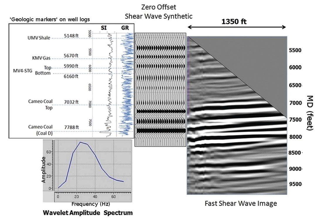
Also, the GR log shows that the depth interval of 5400 ft to 6500 ft is comprised of sandy zones. It is expected that in the well 441-20 the sandy depth interval should have higher amplitudes than a depth interval predominantly comprised of shale (6500 ft to 7000 ft). In the VSP image we observe the expected higher amplitude response in the depth interval of 5400 ft to 6500 ft and weaker response in 6500 ft to 7000 ft. Then we observe high amplitude response from 7000 ft and below because this is a coal interval and coal has a high shear impedance contrast with either of the sand and shale lithologies present in the Cameo Coal interval.

VSP Image Tie with the Surface Seismic Stacks

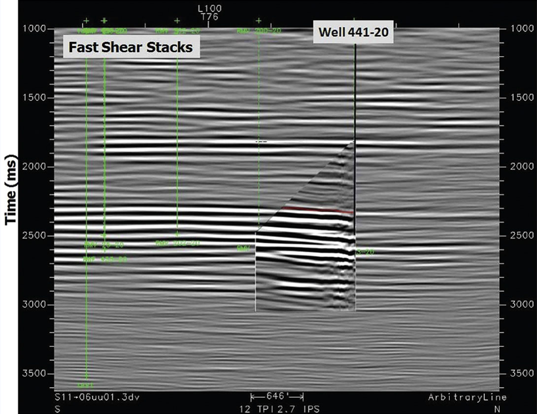
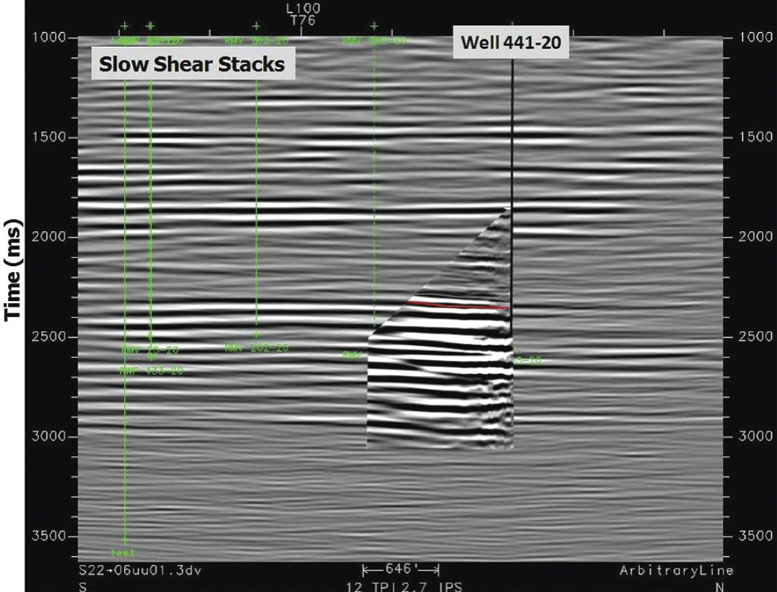
Now let us evaluate the integration of available surface seismic shear wave stacks with their VSP equivalent stacks. This integration is either done by converting the VSP depth images into timedomain images or converting the surface seismic stacks to depth. The VSP images were converted to time domain because we have a calibrated velocity model for the VSP for depth to time conversion. Conversion of VSP depth stacks into time domain shall also help in comparison of their temporal frequency. The conversion to time domain is done by using V^‖_S0 and V^┴_S0 to the fast and slow VSP depth images respectively. Figure 4 shows the overlay of the fast shear wave VSP stack (foreground) on the fast shear wave surface seismic stack (in background). Figure 5 shows the equivalent overlay of the slow shear wave stacks. It is worth mentioning that most of the major reflectors (Cameo Coal interval and below) in the surface seismic tie with their VSP responses. The VSP-surface seismic tie enables joint study of the two datasets for subsurface evaluation.

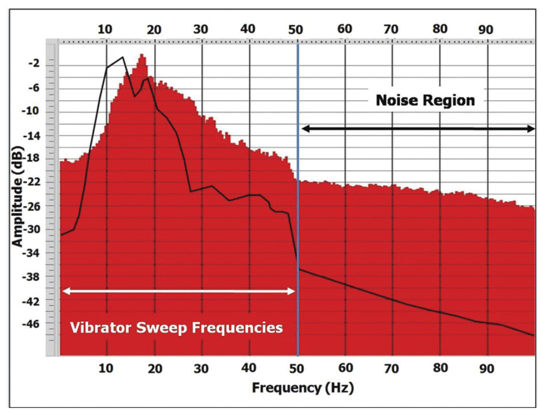
The amplitude spectrum of the fast VSP stack and the fast shear wave surface seismic stack is shown in Figure 6. As expected the VSP data has larger bandwidth of signals than its surface seismic equivalent and hence improved temporal resolution.

Evaluation of the Pay in Williams Fork Formation

In the previous sections we established the agreement between the fast and slow VSP stacks in terms of reflector depth positioning. It was also demonstrated and explained how the well 441-20 ties with the VSP stack. Next, we evaluate the reservoir section in the Williams Fork Formation on the VSP stacks. It is evident in Figure 3 that we have depth dependent lateral coverage of the subsurface in a walkaway (or long offset 3D) VSP survey (Kohler & Koenig, 1986). In the VSP survey at well 441-20 we can evaluate the depth interval of 6000 ft and deeper. As shown in Figure 3 this depth interval shall have a lateral coverage of 700 ft (at measured depth of 6000 ft) to 1350 ft (at measured depth of 7250 ft and below) in all directions.

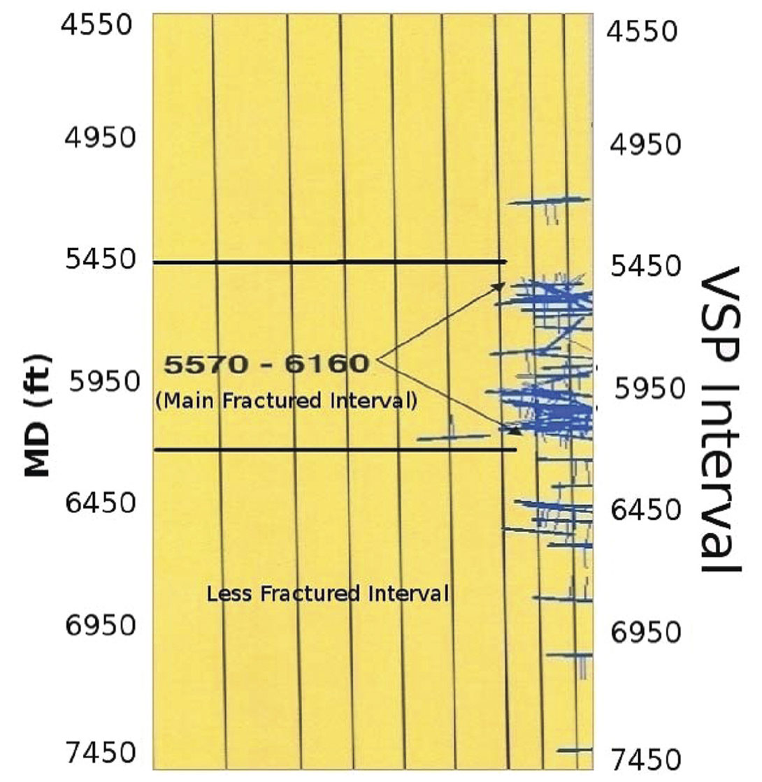
Starting from the GR log in well 441-20 the measured depth interval of 6000 ft to 6200 ft suggests a sandy interval (with lower GR values) with thin sands (total sand thickness of 150 ft) intercepted by the well 441-20. RMS amplitude map corresponding to this depth interval is computed and the results are shown for both fast and slow VSP images in Figure 7.

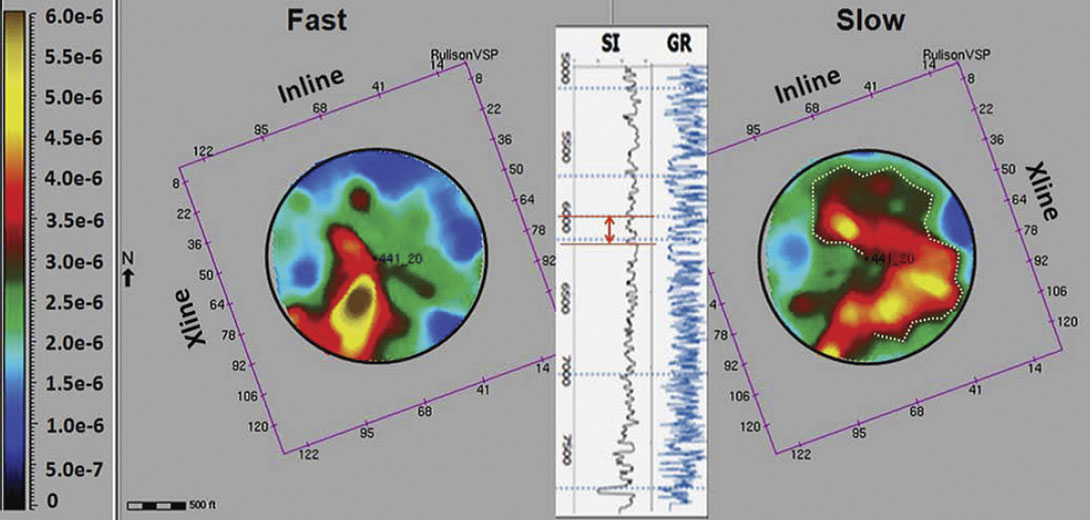
The fast and slow VSP images have a different amplitude response at certain zones. Except near the well 441-20, the difference in amplitude arises from the fact that the reservoir is fractured and the reflection coefficients are different for both the non-converted shear modes. Crack density, e, influences the anisotropy parameter (γ_s) that controls the reflection coefficient of the two non-converted shear modes. It has been pointed out in many papers (see Bakulin et al. (2000) for a review) that the shear-wave splitting coefficient is close to the crack density, g^(v) ~ e. Inference of crack-density estimates from shear wave reflection amplitudes requires the normal-incidence reflection coefficients and is not the objective of this study.

The portion of the map marked with white dots on the slow shear wave VSP stack (Figure 7) indicates areas interpreted to have intense fracturing. Fractures decrease impedance of slow-shear waves giving rise to higher RMS amplitude. In Figure 7 the fast shear wave VSP image shows the sandy interval (RMS values of 3.0e-6 and above). The well 441-20 apparently did not hit the thickest portion of the sandstone body at this depth. This same observation can be made from the slow shear wave VSP stack.

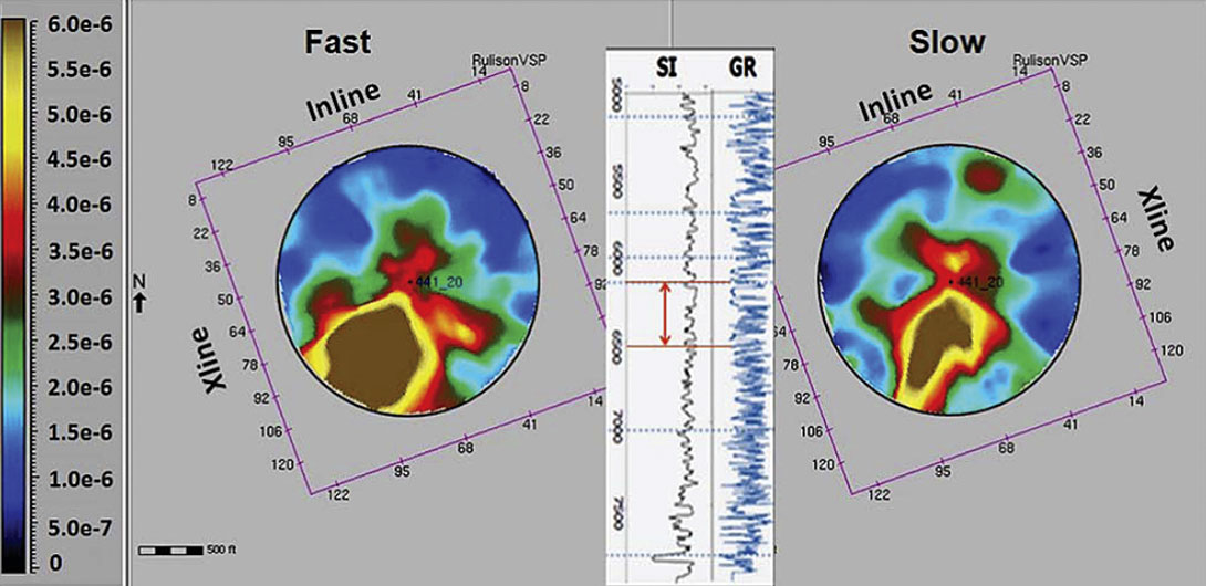
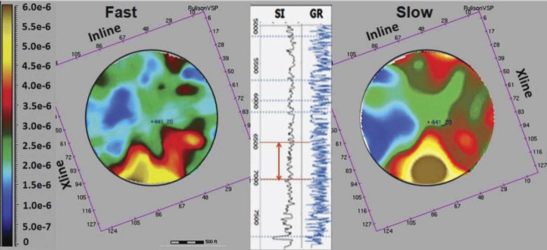
Figures 8 and 9 show the RMS amplitude maps at reservoir depths of 6200-6500 ft and 6500-7000 ft respectively. The inset in Figure 8 shows that the well 441-20 has intersected thick sand units (about 250 ft) from 6200-6500 ft. The RMS amplitude values at the well location are similar (about 3.5e-06) for both the fast and slow VSP stacks. This may suggest that the sand is devoid of fractures at this depth interval (in 6200-6500 ft interval). Similar observations can be made from the fracture interpretation of the FMI log in well 441-20 (Figure 10). Figure 9 shows the RMS amplitude map extracted at 6500 ft to 7000 ft which corresponds to a predominantly shale interval in the well 441-20 (inset in Figure 9). The well 441-20 did not encounter any sandstone in this depth interval. The sandstones are present south of well 441- 20 from the VSP image.

Fault Interpretation

Strike-slip faults or wrench faults are the main cause of tectonic fracturing at Rulison Field. Strike-slip faults form in response to horizontal shear movement within the subsurface. Strike-slip faults are characterized by a linear or curvilinear displacement zone in plan view (Christie-Blick & Biddle, 1985; Kuuskraa & Hansen, 1997) suggested that fault planes terminate within midpay sections and splay into a wedge of fracture systems characterized by reflector offset, amplitude dimming, and generally poor amplitude coherency. They observed that near the faults there are more likely to be natural fractures and greater well productivity.

Apart from detecting the stratigraphic details VSP images are also capable of showing faults in the subsurface. Use of P-wave VSP images for fault detection has been reported in literature (Gras & Craven, 1998, Chavarria et al. 2007). The use of VSP images specific to tight reservoirs in Jonah Field in Wyoming is documented by House et al. , 2009) where they demonstrate that in spite of the VSP well being uneconomic the recovered VSP images in the field allowed better understanding of the faults that control gas production. The improved understanding of the fault features resulted in later exploration successes. In Rulison Field detection of such fault features is important because the rocks close to such fault features are generally fractured and contribute to high permeability conduits to the wells that intersect such fractured zones. Fractured zones have resulted in higher gas production in Rulison Field (Matesic, 2007; Rojas, 2008). Because the formation is hydraulically fractured it is important to identify these faults because during hydro-fracturing fluids can escape through such fault planes thus making the treatment less effective.

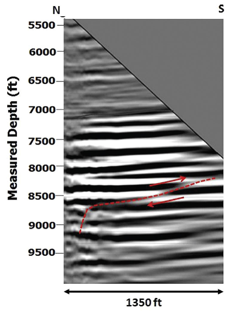
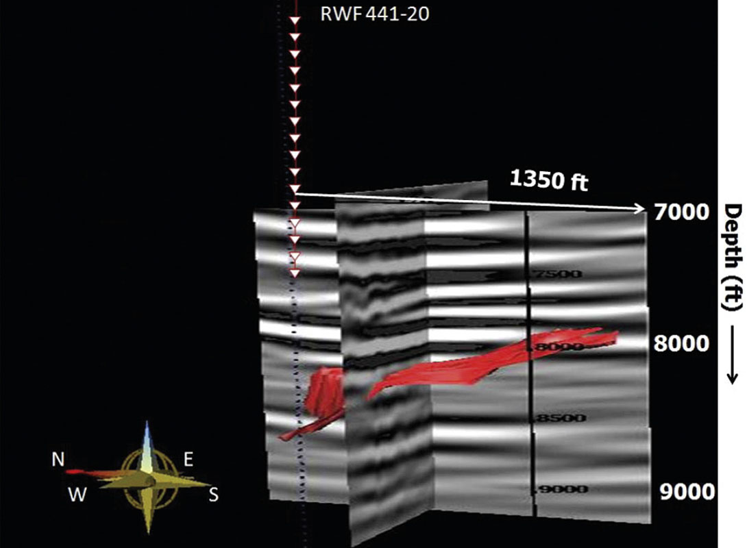
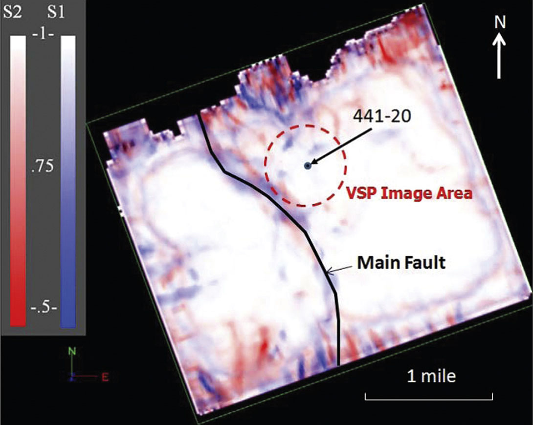
In the 2006 VSP survey one fault feature can be identified on the south-west portion of the imaged area and is shown in Figure 11. The fault feature can be identified on many lines in the VSP image. The three-dimensional view of the identified fault is shown in Figure 12. The identified fault on the VSP image could be a fault splay connected with the main North-South trending fault (shown in Figure 13) or could be a part of an altogether different flowerstructure (Cole & Cumella, 2003) known to exist in fields within Piceance Basin. The fault feature identified on the VSP image is not observable on the surface seismic stacked data and such low-angle fault features are difficult to identify on FMI logs.

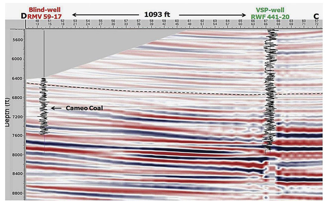
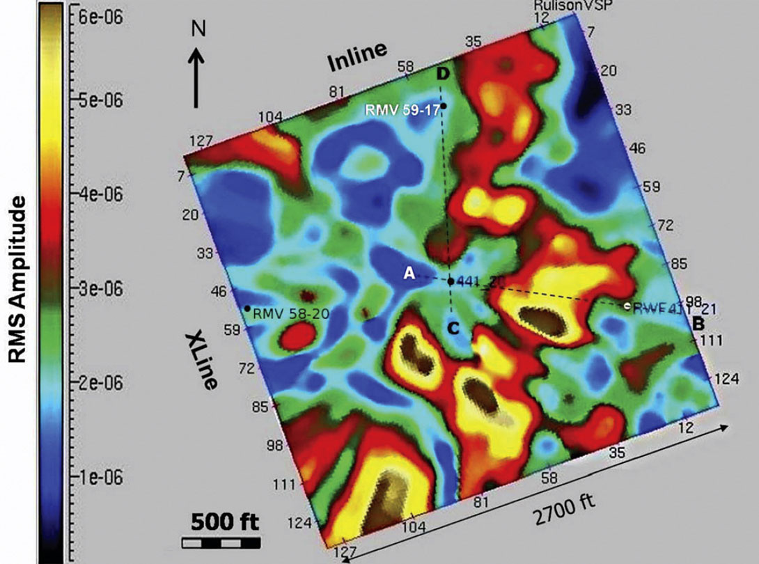
Blind-well Test

Other drilled wells in the VSP image area are put on the map to study the spatial variation of lithology intersected by the wells. This procedure, called the blind-well test, uses well results that can test the validity of the VSP migration results away from the VSP well location. Wells RWF 411-21, RMV 58-20 and RMV 59-17 drilled away from the VSP well 441-20 are shown in Figures 14 and 15. The seismic line, AB, connecting the wells 441-20 and RWF 411-21 is shown in Figure 14 and, line CD, connecting 441- 20 and RMV 59-17 is shown in Figure 15. A seismic reflector identified on well RWF 411-21 (marked by black dashed horizon shown in Figure 14) corresponding to a top of sandstone layer, MV1 (STG TOP), is interpreted on the VSP image volume. The continuation of the same reflector passing through wells 441-20 and well RMV 59-17 is shown in Figure 15. A RMS amplitude map, extracted with an 80 ft window centered at the interpreted horizon, is shown in Figure 16. The gamma-ray logs on seismic lines in Figures 14 and 15 shows that the VSP well 441-20 intersects shale, the wells RMV 59-17 and RWF 411-21 intersects thin sandstone respectively. The well RMV 58-20 is at the edge of the VSP image and does not have high-quality amplitudes to carry out the blind-well test. None of these wells hit the high-amplitude sandstone bodies shown in Figure 16. The VSP image can thus be used as a tool to plan successful wells within the image area.

Conclusions

The non-converted shear wave reflections as recorded by VSP geophones provide higher resolution images (as compared to the surface seismic data) in the main gas interval in Williams Fork Formation and the underlying coal layers in Cameo Coal interval. The improved image quality from VSP recording is attributed to its broader bandwidth as well as to low noise environment as compared to surface seismic recording. Better resolution of VSP data enables the location of stratigraphic features like sandstoneprone intervals and pinchouts in coal beds. Additionally, VSP images detect structural elements like fault features (not visible on surface seismic data). Presence of fault features is important to know because drilling through faults can result in poor performance of the well. However, drilling close to such features can result in high production rates because the rocks close to such faults generally have higher fracture density.

Acknowledgements

The authors thank sponsors of RCP and RPSEA consortium for research funding. We appreciate help extended by Williams Production Company that allowed us to do the blind-well tests in our study.