Skeletonization and Empirical-Mode Decomposition of 2-D Potential-field Images

The volumes of modern gridded data collected by the geophysical exploration industry are often large and can benefit from methods for image decomposition, pattern analysis, and interpretation. Automated pattern-recognition methods can be useful for both seismic and potential-field images. In both of these cases, it is important to extract quantitative attributes useful for further data analysis and inversion for the subsurface structure. In this paper, we investigate one of such pattern-analysis approaches called “skeletonization”.

Although using different physical fields and models, many types of 2-D geophysical images, such as seismic sections and slices, gravity and magnetic maps, possess a number of similar geometrical features. These features can be expressed by linear continuity, branching, amplitudes, widths, polarities, curvatures, orientations and/or other attributes and can be subdivided into “background trends” on top of which some kinds of “anomalies” or “wavelets” can be recognized. The types of spatial dimensions of the images may also vary, ranging from the usual distances, elevations and depths to travel times and travel-time lags. Automatic identification of such spatially-connected wavelets and measurement of their parameters is the general objective of skeletonization.

This paper describes a new, azimuthally-uniform skeletonization approach to 2-D potential field data. The majority of the material in the following sections was originally published as Paper A-3 in Summary of Investigations 2012, Volume 1, Saskatchewan Geological Survey Miscellaneous Report 2012-4.1 (Gao and Morozov, 2012). This material is reproduced here, with modifications, with permission from the Saskatchewan Geological Survey.

Introduction: Seismic and Potential-field Image Skeletonization

The original development of the skeletonization technique targeted automatic event picking in reflection seismic data (Le and Nyland, 1990; Lu and Cheng, 1990; Li et al., 1997). In these approaches, pattern primitives, such as wavelet amplitudes, durations and polarities, were extracted from seismic traces and connected along the offset dimension according to certain similar features to form a coherent event. Starting from the stronger seismic-reflection events, weaker events were identified and connected iteratively. This technique was based on the so-called binary consistency-checking (BCC) scheme by Cheng and Lu (1989); however, the use of any particular ranking scheme is not important for skeletonization. More recently, Eaton and Vasudevan (2004) extended this method to aeromagnetic data by using detection on the basis of strike direction, event linearity, event amplitude and polarity.

When applied to gridded potential-field data maps, a significant drawback of seismic-algorithm based skeletonization consists in one direction being preferred and treated as reflection travel-time. In the applications of such algorithms to potential-field grids described by Eaton and Vasudevan (2004), this problem was alleviated by making two passes of pattern analysis. During the first pass, the Y direction (north) was treated as the “time”, and prior to the second pass, the grid was transposed and the X direction (east) was treated as the “time”. Thus, the structural features were still detected and connections made predominantly in two orthogonal directions within the image. This scheme is non-uniform azimuthally and may be biased toward the gridlines of the images, resulting in potential “footprints”. In addition, the basic wavelet used by Eaton and Vasudevan (2004) was of a near-zero mean, bipolar “seismic” type, which consisted of a peak followed by a trough. This wavelet may be well suited for certain types of magnetic sources (such as dipping magnetic sheet) but it still appears to be too specific for the more general feature detection needed for analysing unipolar potential fields or amplitude variation with offset (AVO) patterns in pre-stack seismic applications. A low-frequency background with nonzero mean can thwart feature extraction and cause disruptions in the “skeleton”. Pre-filtering of the image prior to event detection could also be undesirable, as this could complicate processing and cause loss of information about the background trends.

In this paper, an approach opposite to that by Eaton and Vasudevan (2004) is taken, and a skeletonization technique is developed for arbitrary two-dimensional (2-D) gridded data. Pre- or post-stack seismic sections are only considered as special (although important) cases of grids with specific treatment of the time dimension and also (potentially) additional constraints and attributes. While achieving the same general goals of quantitative recognition of linear features in gridded images, this technique is highlighted by the following properties:

1. Feature detection performed isotropically, at a continuous range of azimuths (or time-distance moveouts if the image is a seismic section);
2. Several new features, such as extraction of orientation angles and background-trend level, are used to meet the complexity of the data; and
3. A more flexible event detection scheme is used instead of the BCC method.

An important advantage of this algorithm is in its integration in a powerful seismic, well-log, and potential-field data processing system (Morozov, 2008). Numerous signal-processing tools can be included in the image-skeletonization flow, and the user interface allows utilizing many processing and plotting options. In particular, the skeletonization is combined with empirical mode decomposition (EMD) (Morozov, 2009), which allows emphasizing different-scale structures and exploring them for multiple attributes and purposes.With additional new options and “on-the fly” wavenumber filtering during the background-trend extraction (next section), the algorithm also provides stable (with respect to variations of the potential-field background) identification of structural features.

Method

Similarly to the previous approaches (e.g., Eaton and Vasudevan, 2004), the image skeletonization in the present method is achieved in two general steps: 1) identification of elementary “anomalies”, or “wavelets” in gridded images, and 2) connection of these wavelets to form the “skeleton” of the image. In seismic sections, the skeleton can be interpreted as a set of “horizons”, and in the potential-field case, it comprises any “lineaments” (elementary linear and potentially branching features) detected in the image. Each of these “lineaments” is associated with a set of parameters referred to as the “feature set” and can be interconnected with other “lineaments”.

Wavelet Detection and Feature Extraction

Starting from a grid of “seed” points located on the vertical and horizontal cross sections, pattern primitives called “wavelets” in the 2-D grid are identified as combinations of one or two amplitude deviations from the background trend level (Figure 1). In this paper, these unipolar deviations are referred to as “humps”. From each seed point, the humps are first searched within the cross-section line, and then their final locations and orientation azimuths are determined by minimizing the cross-sectional sizes (distance AB in Figure 1a). With the option of subtracting the slow-varying trend, the humps are identified even on top of a slowly varying amplitude background (long-dashed grey line in Figure 1b). Several other user-selected options are available for the wavelet-extraction algorithm. In particular, waveform edges may be identified by the locations at which their amplitudes pass through the smoothed background level (points A and B in Figure 1) or by using zeros of second derivatives (inflection points) of the signal. These options may be useful in the presence of strong-background (as common in magnetic data) or short-wavelength noise in the records.

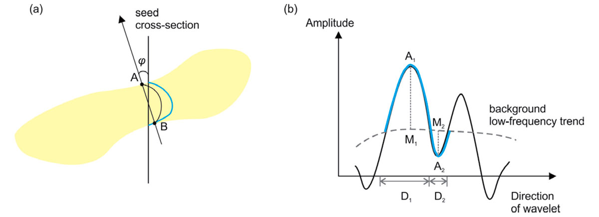
Once the wavelets are isolated, their polarities and spatial directions are determined by comparing the two humps within them (similar to Eaton and Vasudevan, 2004) or also by comparing the amplitudes of adjacent wavelets. “Undefined” values of polarities are also allowed in cases where they cannot be determined with sufficient confidence.

For subsequent pattern analysis, the wavelets are characterized by their peak or trough amplitudes (A₁ and A₂), widths (D₁ and D₂), orientation angles (φ), background levels and polarities (P; Figure 1b). Combinations of these parameters represent the desired feature sets:

Wavelet connections

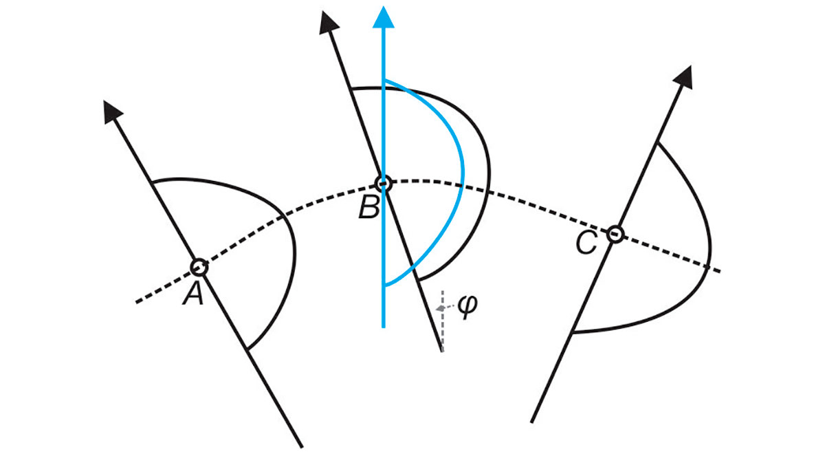
After all wavelet features are determined, they are spatially connected to form the image skeleton. This process is started from either: 1) wavelets manually picked by the user or 2) wavelets with the largest amplitudes. First, each selected wavelet is connected to several adjacent wavelets according to the lowest connection costs. The cost function for connection is designed to evaluate the similarity of two wavelets and their spatial proximity. For example, for humps A and B, the cost function is (Figure 2):

where r^A and r^B are the spatial coordinates, f^A and f^B are the corresponding feature vectors (1), and w_i are some empirically-determined weights.

Among all pairs of potential connections, optimal triplets are further identified. For example, for wavelet B in Figure 2, several candidates for adjacent connections A and C are considered based on the orientation angle,φ. Among these candidates, the optimal pair is found by minimizing the following connection-cost function:

where interp(B) (blue line in Figure 2) is the feature set (wavelet) interpolated at location B by using wavelets A and C. The interpolation is based on the mutual cost functions for pairs of wavelets, Cost(A,B) and Cost(B,C). Note that this triplet connection scheme does not use the somewhat arbitrary Euclidean distance and area-of-triangle principles used by Li et al. (1997) but measures the similarity of wavelets directly by their zero-lag cross-correlation (Figure 2).

Empirical Mode Decomposition

Prior to identifying the wavelets and features in a 2-D image, it is useful to decompose the image into components containing different scale-lengths. Such decomposition can be performed by the process called Empirical Mode Decomposition (EMD; Hassan, 2005). The EMD is in an iterative procedure that sequentially extracts 1-D or 2-D dependences called “empirical modes” from the data, so that the sum of all modes represents the original signal. In a one-dimensional case, starting from a data record, u(x), the first empirical mode u1(x) and its residual r1(x) are determined:

and the residuals are further decomposed recursively (n = 1,2…):

When the coordinate x is the time and u_n(x) are time series, Hilbert transform is used in these equations to extract the “upper” [E_u(x)] and “lower” [E_l(x)] envelopes of the signal, and the corresponding n-th empirical mode u_n(x) is defined as their average (Hassan, 2005):

This operation produces a low-frequency signal following the averaged trend of u(x). However, this procedure only works for oscillatory signals such as seismic waveforms, for which E_u(x) and E_l(x) are always positive, and negative, respectively. In 2D, and particularly for potential-field data with a significant background trends in large areas, this assumption fails, and the Hilbert transform does not allow obtaining consistent E_u(x) and lower levels E_l(x) bracketing the signal.

To overcome the above difficulty, Morozov (2009) proposed a simple type of EMD without the need for Hilbert transforms. This procedure is applicable to an arbitrary number of spatial dimensions and does not require some of them having the meaning of “time”. Instead of eq. (6), the nearest empirical mode is defined as:

where F_k[…] denotes low-pass filtering with cut-off wavenumber k. Starting from k = 0 (with n= 1), the value of k is gradually increased until the average amplitude of un exceeds a small portion (e.g., 5%) of the amplitude or r_n-1. This iterative procedure achieves the goals of EMD by effectively constructing a series of band-pass filters in wavenumber k, so that each filtered component (except the original one with n = 0) contains an approximately equal portion of the total energy. As required by the EMD principle, the decomposition of the 2-D signal is controlled only by the signal itself and performed isotopically, i.e. independently of the orientations of the grid axes.

Results

In this section, examples of aeromagnetic and gravity are used to illustrate the application of 2-D of skeletonization and its use with EMD algorithms.

Aeromagnetic data examples

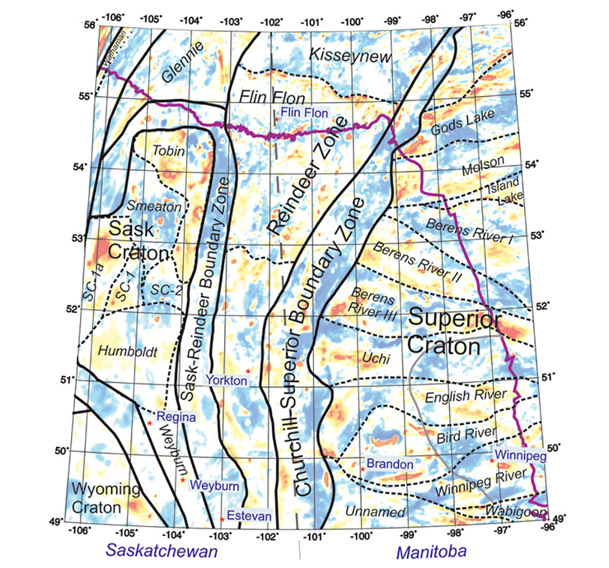
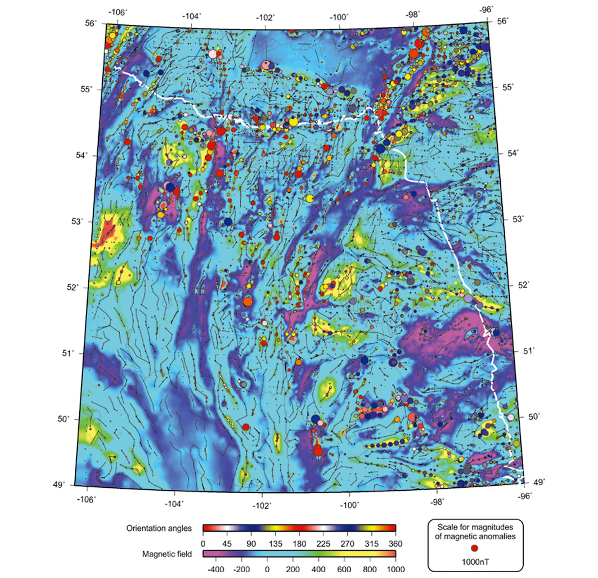
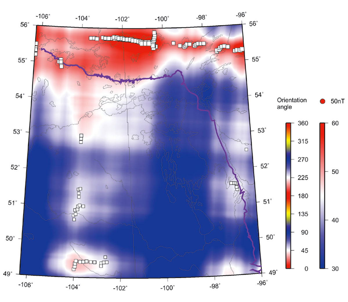
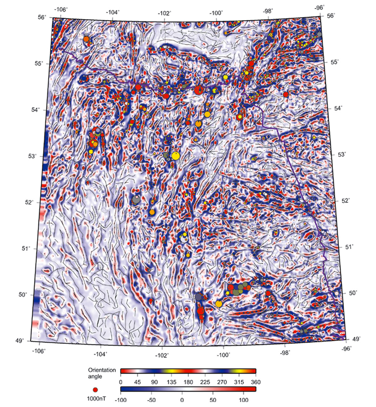
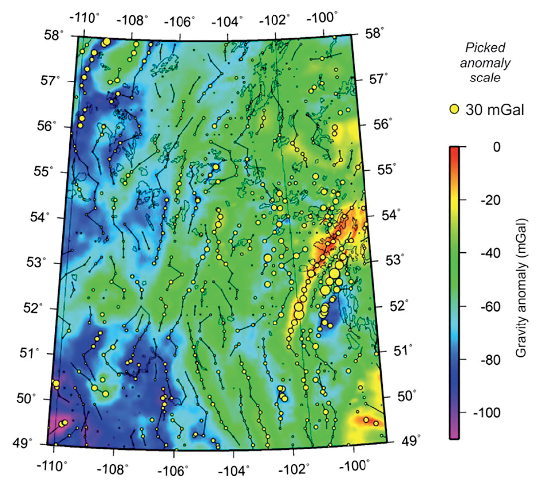
First, let us consider examples of regional gridded magnetic-field data from southeastern Saskatchewan and southwestern Manitoba (Gao and Morozov, 2012). The study area extends from W96º to W106.3º and from N49º to N56º (Figure 3) and was a part of the Phase 2 of the Targeted Geoscience Initiative (TGI2) project focusing on the Williston basin (Li and Morozov, 2007). Figure 4 shows the aeromagnetic data obtained from Natural Resources Canada after basic pre-processing and reduction to the pole. In this and other images, the major geologic structures and geographic references can be identified by comparing to Figure 3. In NE parts of this and the following Figures, the long “wiggly” lines show the edge of the exposed Canadian Shield.

On top of the magnetic grid, Figure 4 shows the results of skeletonization using this raw grid with spatial demeaning within a 30-km sliding spatial 2-D window. Coloured circles indicate the picks of major features and black lines indicate linear anomalies connecting the features (the skeleton). The identified anomalies are indicated by circles with sizes proportional to the absolute values of demeaned amplitudes. Colours of the circles correspond to the orientations of the anomalies, defined as the directions in which the cross-sections of the anomalies are the most compact. These angles are thus always oriented across the structure and measured from the eastward direction toward the North (upper colour bar in Figure 4). As Figure 4 shows, skeletonization identifies numerous linear elements of the structural fabric of the region, even those which can hardly be recognized visually from the original grid. However, many “seed” picks remain disconnected and look like isolated dots in Figure 4 because of the strong regional bias in the amplitudes in this raw map.

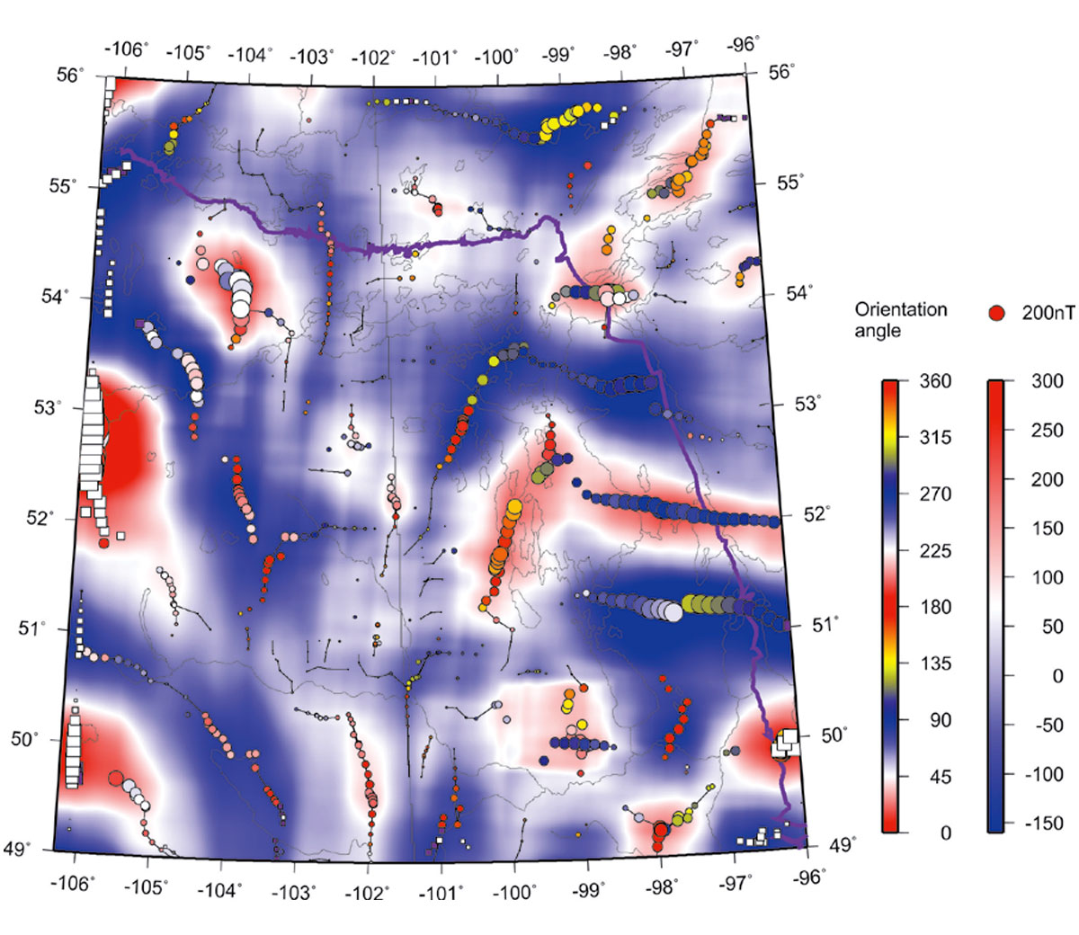
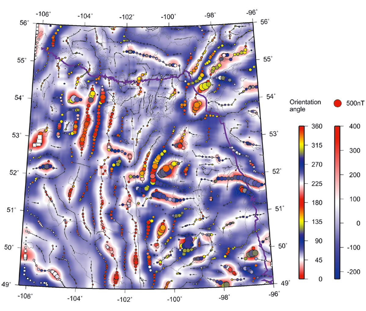
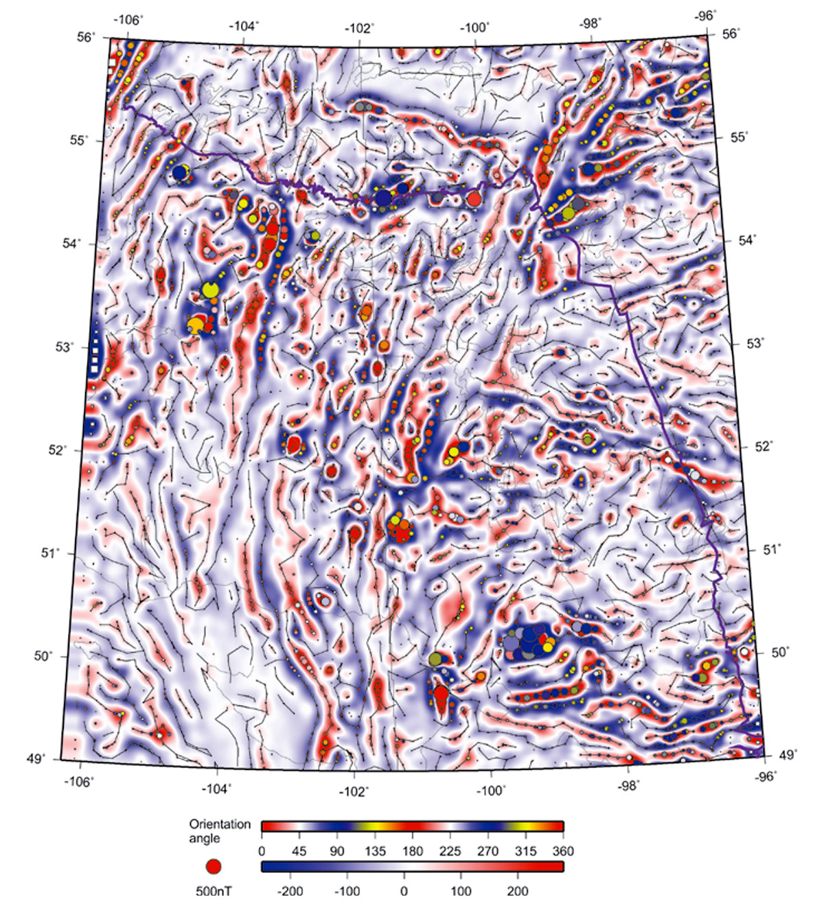
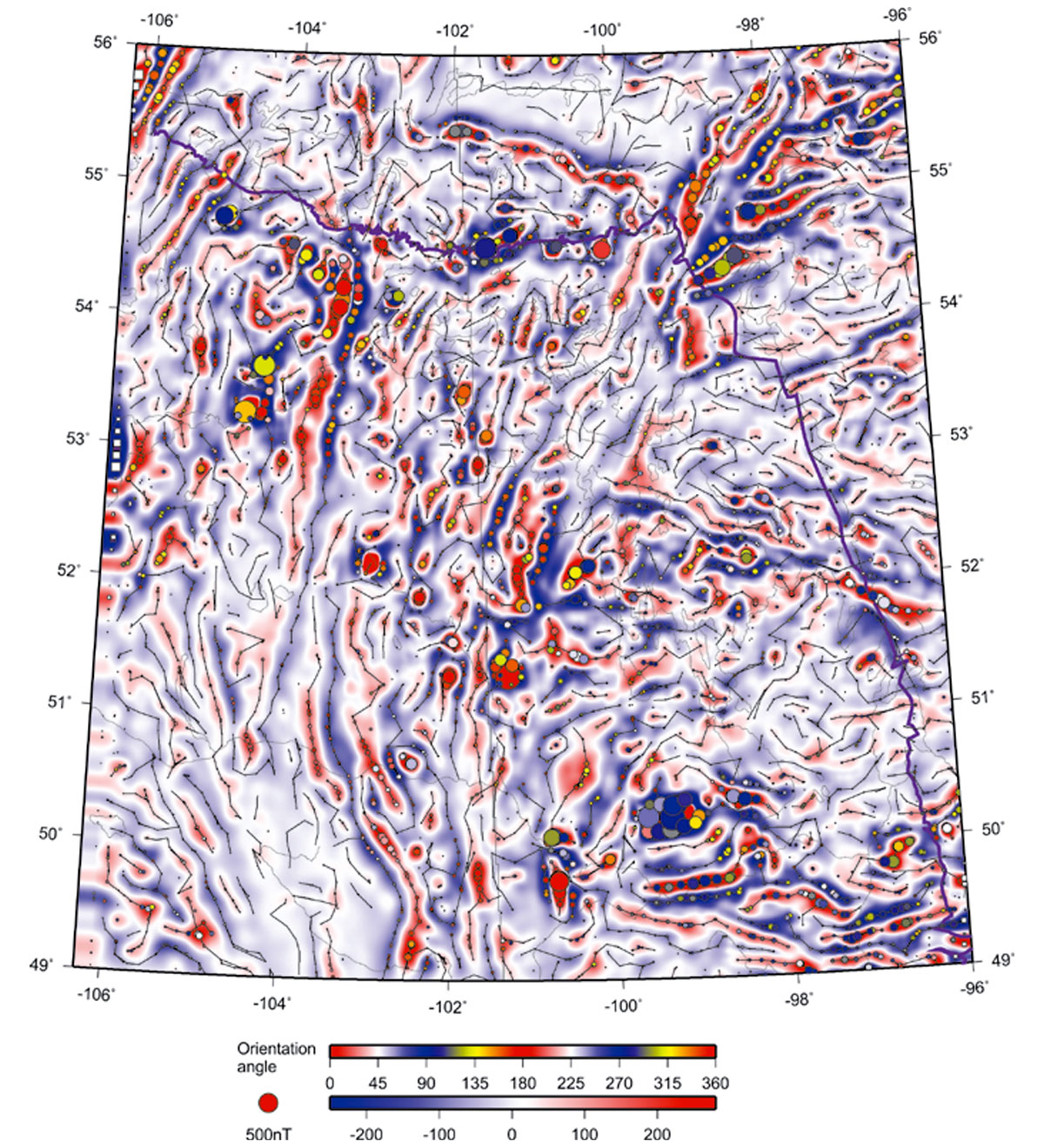
Figures 5 through 10 show decompositions of the magnetic grid into several “modal” fields by using the 2-D EMD technique outlined in the preceding section. These modes represent results of progressive low-pass filtering, so that each mode possesses a certain spatial scale length, and the sum of all modes again reproduces the original field in Figure 3. Each of these empirical-mode images is skeletonized in a way similar to shown in Figure 3. In these EMD-filtered images, note the dominant linear trends of picked events, which are mostly SW-NE in the northern parts of the images and NW-SE in the southern areas.

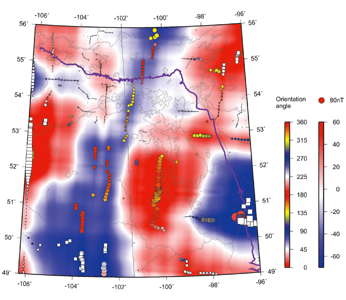
The “skeletons” of the images also include the amplitudes of the anomalies, which are indicated by the sizes of coloured circles in these Figures. Purple circles are anomalies with negative “polarities” (i.e., proximities to other anomalies of lower magnitudes; Eaton and Vasudevan, 2004), and white squares indicate the anomalies to which no definite polarities were assigned.

The skeletonized EMD images are useful for refining the boundaries of the geologic domains and sub-domains. Figure 11 shows EMD component with n = 6 (highest-resolution) superimposed over the identified domain boundaries (also shown in Figure 3; Li and Morozov, 2007). Generally, the boundaries match with the contours of this empirical mode, although some areas contradictions are also found, such as indicated by question marks in Figure 11. The placements of block boundaries in these areas may likely need to be revisited in the future, possibly with the use of the obtained image skeleton and additional gravity and aeromagnetic attribute maps (Li and Morozov, 2007).

Once the image is decomposed into wavelets, features extracted and the skeleton created, its spatial attributes can be analysed in many ways. Figure 12 shows the skeleton images filtered by the lengths and angles of its near-linear features. Note how the lengths and orientations of near-linear features vary for different parts of the study area.

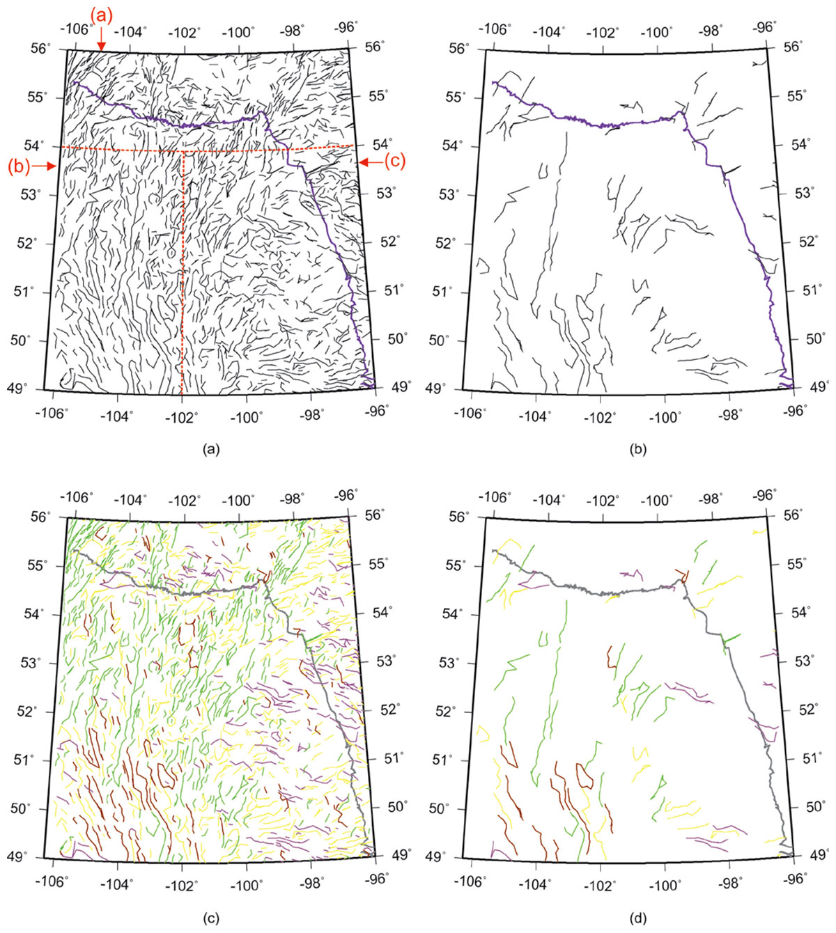
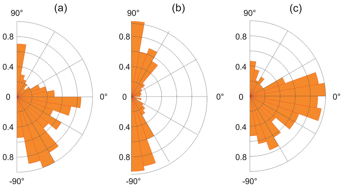
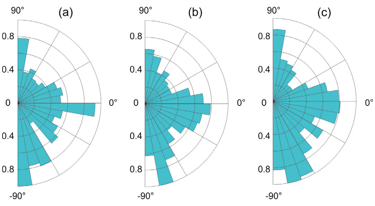
Rose diagrams in Figure 13 summarize the strike directions for the linear anomalies picked from three different scales of the EMD. As noted above, lineations striking at about N-S and E-W directions dominate these images. In Figure 14, I also show the azimuthal distributions of the features detected in the highest-resolution EMD component n = 6 for three areas: (W96º –106.3º, N54º –56º), (W102º –106.3º, N49º–54º), and (W96º–102º, N54º–56º), indicated by labels (a)-(c) in Figure 12. As Figure 14 shows, the first of these areas is heavily dominated by lineations striking at ~10º and ~70º south of the eastward direction; in the second area, the lineations are almost N–S, and in the third, they are dominated by the E–W direction.

Gravity data example

To illustrate application of skeletonization to gridded gravity data, the TGI2 study area is the same as for magnetic data examples (Figure 3). Similarly to the preceding images, gravity skeleton (Figure 15) shows dominant linear structural trends, which are SW-NE and complementary to the magnetic trends. Consequently, the features detected in the gravity image could be utilized in a joint interpretation of the basement structure in the study area (Li and Morozov, 2007). Similarly with the aeromagnetic images, Figure 15 also shows dominant linear event trends, which are SW-NE in northern parts of the study area and NW-SE in the south. The skeleton of the image also contains positive anomalies, which are indicated by the sizes of circles plotted in this figure. Due to a different physical nature of the gravity field (unipolar character and slower decay with distance from the source), the spatial detail of the gravity image is significantly lower than that of the magnetic images.

Conclusions

The proposed geophysical skeletonization technique is an effective and useful tool for pattern recognition in 2-D potential-field and seismic images. The process of skeletonization can help to automatically and objectively identify and quantitatively characterize various types of amplitude and directional anomalies. The skeleton represents a convenient and quantitative tool for delineating geological structures in the maps or for auto-picking horizons in 2-D seismic images. Compared with previous methods, this algorithm is more general, isotropic in 2-D feature detection, and applicable to arbitrary gridded geophysical data.

Applications to both potential-field and seismic data interpretation (Gao, 2017) shows that the skeletonization technique could aid in the interpretation of complex 2-D structures. Skeletonization is particularly useful in combination with 2-D Empirical Mode Decomposition. These approaches should be particularly useful for refinement of domain and structuralblock boundaries, identification of lineation patterns, and for inversion of gridded magnetic and gravity data. The technique should also provide a basis for numerous application of 2-D (and in the future, 3-D) skeletonization to improved interpretation of seismic sections and volumes, and also to more advanced AVO analysis in seismic applications.

Acknowledgements

Initial processing and analysis of TGI2 potential-field data was performed by Jiakang Li (University of Saskatchewan).