Recent technical innovation associated with sparse 3D design has resulted in acquisition costs that are substantially lower than both traditional 3D and comparable 2D seismic acquisition expenditures. The Sparse 3D cost/sq. km. price breakthrough has allowed Amoco Canada to pursue Devonian play trends into operationally difficult, heliportable, foothills terrain by acquiring arealy large 3D's over exploration targets for a fraction of the cost of previous surveys. Traditional heliportable 3D surveys in N. America run between $25-70 thousand dollars per sq. km. Various large heliportable Sparse 3D surveys (3000+ sq. km. total area) were successfully acquired over the last few years (1992 to 1997) for an average cost of less than $10 thousand dollars per sq. km. In addition the use of decimation testing has allowed successful expansion of the Sparse 3D technique to structural plays and shallow stratigraphic targets.
The stratigraphic targets for these sparse 3D's are primarily deep (>4km.) Carbonate bank edges, with large thrust fault deformation in the shallower strata. Poor data quality and the high cost of seismic have acted as barriers to exploration on these plays. Sparse 3D has successfully addressed both these problems and has acted as a catalyst for continued pursuit of resource in these areas.
Sparse 3D is most often associated with low fold, and in that limited sense is not new technology. Most companies have attempted low fold surveys, and discovered that the resulting seismic quality degradation precludes worthwhile cost savings. Amoco Canada's version of Sparse 3D design hinges on a number of other insights, which when exploited, yield cost efficiencies well beyond previous conceptions.
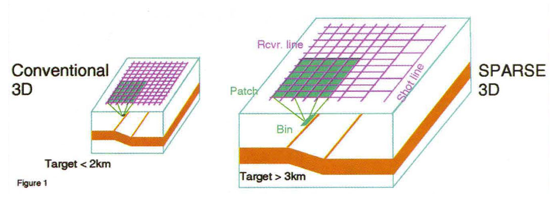
The first insight arises from the recognition that deep targets will have a correspondingly large maximum usable offset range. Adjusting the recording patch to make use of all these offsets (and azimuths) permits wide spacing on shot and receiver lines while maintaining reasonable fold (~10). See figure 1. Wide line spacing (~2km apart) reduces line clearing costs and lowers surface effort (and environmental impact). Each shot creates an emergent wavefront of useful reflection energy that is approximately 12 km. in diameter (for a heliportable drilling cost of over $1000. per shot hole!). We adjust our recording patch to capture as much of the emerging wavefront as is technically feasible. This requires recording crews to possess enough equipment to layout 2500+ channels. Using large numbers of channels, with wide receiver line spacing, covering a large area on the surface, means that less shots are required for the same fold, while simultaneously blanketing a large area of the subsurface. Trading more channels for fewer shots works well, both economically and technically. Narrow azimuth 3D acquisition on land is typically not compatible with lower costs.
The second insight relies on the recognition that the target horizon controls bin size choice. The maximum spatial dip and temporal frequency necessary for clear interpretation of the intended target horizon determine the surface shot and receiver spacing. We do not need tight station spacing to capture steep dips and high frequencies from either shallow horizons or noise. In highly structural settings, bin size is usually kept quite small (read expensive). The reasoning behind the choice of small bins is to keep events with steep dips and high (temporal) frequencies from aliasing during the stacking process, and present problems for migration. To avoid this, we can take advantage of the natural variation in shot and receiver line and station positioning to distribute, or scatter, the shot-receiver midpoints throughout the bounds of the stack bin. During stacking this midpoint scatter acts as a spatial filter (straight sum boxcar weights in space are equivalent to a sinc function response in spatial frequency domain) which helps attenuate reflection event dips and frequencies which would otherwise alias on the output stack. Standard CMP stacking acts as a spatial anti-alias filter allowing greater freedom to shoot with larger (less expensive) bins.
The third insight is connected to the nature of our geology. We recognized that both Devonian reefs (the target) and shallower thrusts (the complication) have predominantly similar strike and dip orientation and hence have different spatial sampling requirements in orthogonal directions. This allowed the choice of placing the receiver lines parallel to the dip direction, with a 70m. group interval (the maximum due to equipment constraints), and shot lines parallel to strike with 200m to 360m shot spacing (resulting in far fewer of the brutally expensive shots)!. This forms a natural bin size that is oblong, a configuration much despised by many geophysicists owing to the supposed difficulty with migration. We have found that modern migration programs will tolerate about a 3: 1 ratio in the two bin dimensions before artifacts appear. For natural bin size ratios greater than this (our norm is 4:1) we stack and migrate at 1/2 the natural bin size (and fold) in the larger direction, and sum traces post migration, along strike, to form the original natural bin size (or larger). Fully anti-aliased Kirchoff prestack time migration is able to tolerate even larger ratios without severe artifacts other than frequency attenuation. These approaches may cost a few thousand more in processing, but saves us literally millions of dollars in the field!
The fourth insight relates to our recognition of the distinct advantages available with 3D fold. Our industry holds the general opinion that 3D fold is somehow "better" than 2D fold (e.g., a 12 fold 3D stack is higher quality than a 12 fold 2D stack), but these comments are based largely on empirical evidence. Relatively little information exists which attempts to explain the reasons behind the differences. Full 3D migration, and dominance of far offsets, have both been suggested as reasons, however the slant in favor of 3D fold is apparent prior to migration (on stack data), and attempts to bias toward far offsets in 2D stack do not mimic the gains seen on true 3D. This lack of understanding also leads to misguided (read expensive) attempts to design 3D surveys with uniform fold, and offset/ azimuth distributions that vary smoothly from bin to bin. The "square root of N" signal to noise discrimination works when noise is dissimilar to the signal as well as other noise. When acquiring sparse 3D's, with large recording patches, the 8 or 10 traces that contribute to a single bin are recorded by geophones that can be literally miles apart from each other, similarly the shots that created these traces are also often miles apart. This results in a stack containing traces whose raypaths differ wildly from one another, except for the small portion representing the subsurface reflection point. Abberations or noise associated with the portion of a raypath near a particular shot or receiver will not be repeated on other traces in the same gather because of the wide geographic diversity. Contrast this with uniform 20 shooting, where each trace in a COP has neighboring raypaths that differ by no more than tens of meters. Adding extra shots between existing ones in 20 increases the fold numerically but adds little in the way of noise suppression. The attempt to acquire steep dipping noise without aliasing, to permit filtering in shot and receiver domains in 20, or 30 narrow patch, is fundamentally flawed because a great deal of the shot generated backscattered noise comes from the crossline direction. It is better to attempt to randomize the noise by intentionally aliasing it with wide patch 3D acquisition, and use the power of stack for noise attenuation. Quite simply: you have to cover new real estate by recording to further offsets, or go sideways using crossline geophone arrays or wideline profiling techniques. The recognition that raypath diversity is critical to good S/N enhancement has allowed us to reduce the fold on our sparse 3D's down to the range of 8-12 traces per bin.
The fifth and arguably most important insight is linked to the areal size of the sparse 3D surveys. Faced with a limited acquisition budget, the first 30 seismic parameter to be compromised is typically the size of the survey (of course we would shoot a bigger survey if we had more money). It seems the worst fear of any geophysicist is that they will design a 3D with bins that are too big, or fold that is too low, or near offsets that are too large and end up acquiring an entire survey full of useless data. So fold, bin size, and line spacing are usually chosen very conservatively, at the expense of survey area. The result is a high quality, postage stamp size 3D, with a few properly migrated bins near the middle. It turns out that sacrificing the sacred cows of high fold, small bins and close line spacing. in favor of increased areal coverage, results in three beneficial side effects.
The first benefit is improved migration over a larger portion of the center of the 3D.
As the area of the 3D gets bigger, the ratio of fully migrated interior bins to undermigrated margin grows larger, thus improving the overall quality of the post migration data.
The second, less obvious, benefit of increased size is that the cost of the survey per unit area will decrease. For instance, fixed costs, like mobilization, are amortized over a larger area. More importantly, larger area means that each shot and receiver will have a greater contribution to the overall fold of the survey. This is easier to see if you consider that a shot in the center of the survey, firing into a full recording patch, will have twice as much contribution to subsurface fold, compared to a shot on the edge of the survey which is recorded by only one half of a patch. The shot in the middle of the survey will have four times as much fold value as a shot in the corner of the survey that is recorded on only one quarter of a receiver patch. The same holds true for receivers. Enlarging the 3D survey biases the ratio in favor of stations in the middle compared to stations near the edge. Recognizing that peripheral shots and receivers have less value, and that the edge of the survey is primarily (but not exclusively) designed for migration apron, has led to experimentation with alternate fold distributions on some of the sparse 3D's. By alternately stopping shot and receiver lines short of the survey perimeter (i.e., interlacing), the fold at the edge of the survey will roll in more gradually. See figure 1. This is compatible with migration, as diffraction tails occur deeper in time than the zone of interest, where the stack fold will be higher than the design fold at the zone of interest (as long as the recording patch size is adequate).
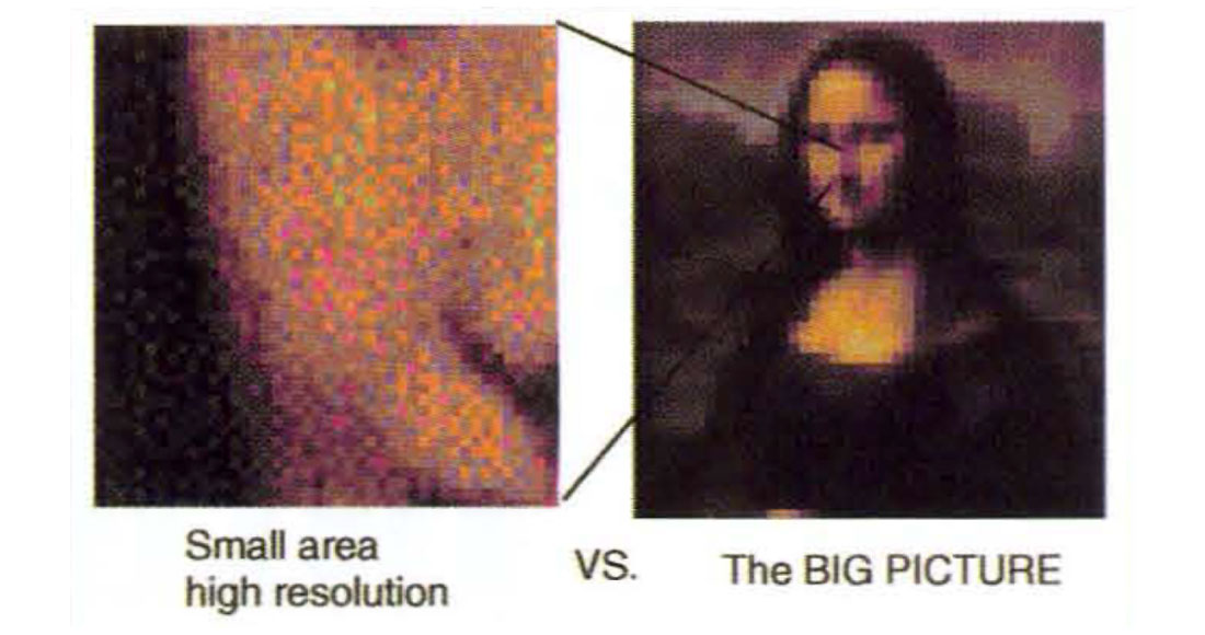
The third benefit of increased size is obvious: you see more of the subsurface. An analogy would be similar to using a close-up 2 inch by 2 inch photo of one of Da Vinci's oil paintings, then trying to guess what the picture was (a grainy large pixel representation of the whole image would be more useful). See figure 2. This has clear advantages for exploration plays.
Amoco Canada exploited the above insights to yield significant cost savings on our 3D acquisition during the 1992-93 shooting seasons. The table below illustrates the cost benefit of using Sparse 3D technology:
Cost comparisons. historical 3D costs for land acquisition (AMOCO)
| Location/type: | Year | Acquisition cost (US $Sq.Km) |
|---|---|---|
| Texas / open land | 1991 | 15275.(range: 13600. - 16900.) |
| U.S. / heliportable drilling | 1980/84 | 52200. (range: 24600. - 87600.) |
| Canada / conventional drilling | 1988/89 | 17000. (range: 12800. - 19500.) |
| Canada / conventional drilling | 1992/93 | 10375. (range: 9750. - 11000.) |
Amoco Canada Sparse 3D surveys:
| Sparse 3D / conventional drilling | 1992 | 4550. (US $/Sq.Km) |
| Sparse 3D / heliportable drilling | 1993 | 5516. (range: 4800. - 6500.) |
The cost comparison table drives home the point that back in 1992-93 the Sparse 3D design was clearly a breakthrough in price performance for Seismic Acquisition. Amoco Canada reserves the title "sparse" only for those 3D's that are less expensive per square kilometer than comparable 2D costs per linear kilometer. In retrospect, some of the insights, such as line spacing scaling with depth, seem trivially obvious today, but received skepticism back in 1992, and currently, exploitation by others is proceeding slowly. These dramatic cost reductions apply largely because the Devonian targets are very deep (more than 4 km). We also developed a way to extend the sparse concepts to shallower targets, and discovered that smaller, but important, cost savings are still achievable.
The initial breakthrough for Sparse 3D in Amoco Canada emerged from a series of processing decimation tests on oversampled 3D surveys. These tests were formalized into a calibrated, empirical approach for determining practical lower limits for future acquisition costs. Amoco Canada typically uses moderately tight spatial sampling, with close line spacing and short group intervals, as parameters for the initial 3D survey in an untested area. This results in a 3D survey with areal extent somewhat undersized, but parametrically overshot. Subsequent simulation of lower priced acquisition schemes can be readily tested during processing, yielding a far better understanding of how quality varies with cost. Additional 3D acquisition in the same area can proceed with parameters that are both adequate and economically viable. This in turn allows areal extents that are larger, and better suited for exploration targets.
This decimation testing allowed Amoco Canada to extend the Sparse 3D concept to both shallower stratigraphic targets and foothills structural plays. The first example of this is a stratigraphic target. shown in figures 3 through figure 6.
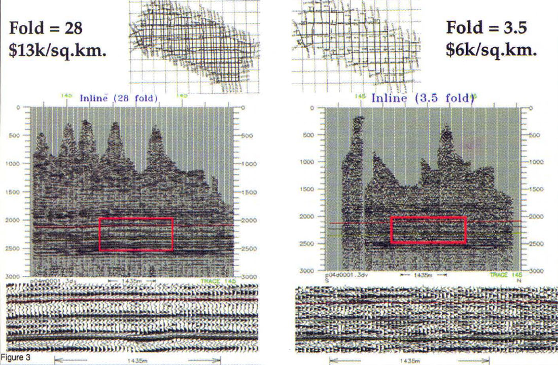
The left portion of figure 3. shows shot and receiver line layout for a 3D dataset from Alberta. The survey was acquired with tight line interval, resulting in a high degree of capture for the emerging reflected wavefronts, and attendant high fold. The right portion of figure 3. shows the line layout for the same dataset after severe decimation of the surface coverage. Here surface sampling, and subsurface fold, were reduced to one eighth of the original acquisition, by omitting half of the shot lines, half the receiver lines, and deleting every second station on the remaining shots lines. This decimation was applied in the initial stage of processing, as if the tapes were received from the field containing less data. The full processing sequence was repeated for this decimated survey, including new statics, velocity analysis, and migration.
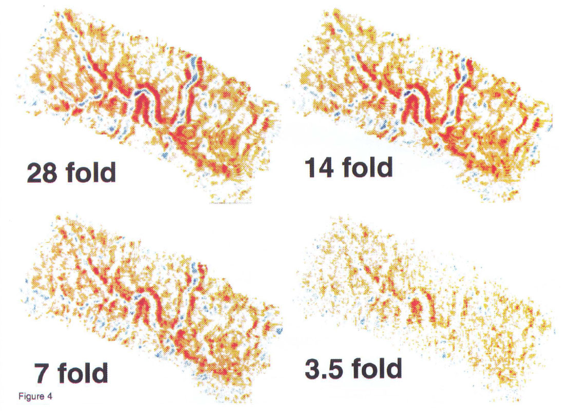
Armed with only the information visible in the pair of wiggle trace seismic sections of figure 3. our simple conclusion would be that reducing surface effort to such a low level would be unacceptable by any interpretation standards. Recognizing that various play types have different interpretation requirements prompts further investigation. Time slices from the above decimation tests, along with two additional intermediate decimations, are shown in figure 4. Each 3D volume was produced by simulating a different level of surface effort. which allows for convenient discrimination of the four time slices with the unitless label of subsurface fold. In each case the processed bin size and maximum offset were kept constant, making the variations in fold proportional to surface sampling. The four time slices in figure 4. show that the data quality of this 3D survey consistently degrades with reduced surface effort. The time slices also show that the evidence of a paleo-drainage system is remarkably robust, and remains visible (albeit noisy) even at very low fold levels.
This test suite is an invaluable method for determining the level of S/N that can be tolerated without masking critical interpretation features. The choice of surface effort is not universal, and requirements will vary depending on which of the features are necessary to locate a well. If only the rough shape of the meander is required than 4 fold may be enough, but if subtle amplitude variations make the difference between good and bad wells then 20 fold may be the lower limit. Processing tests such as these make that determination possible.
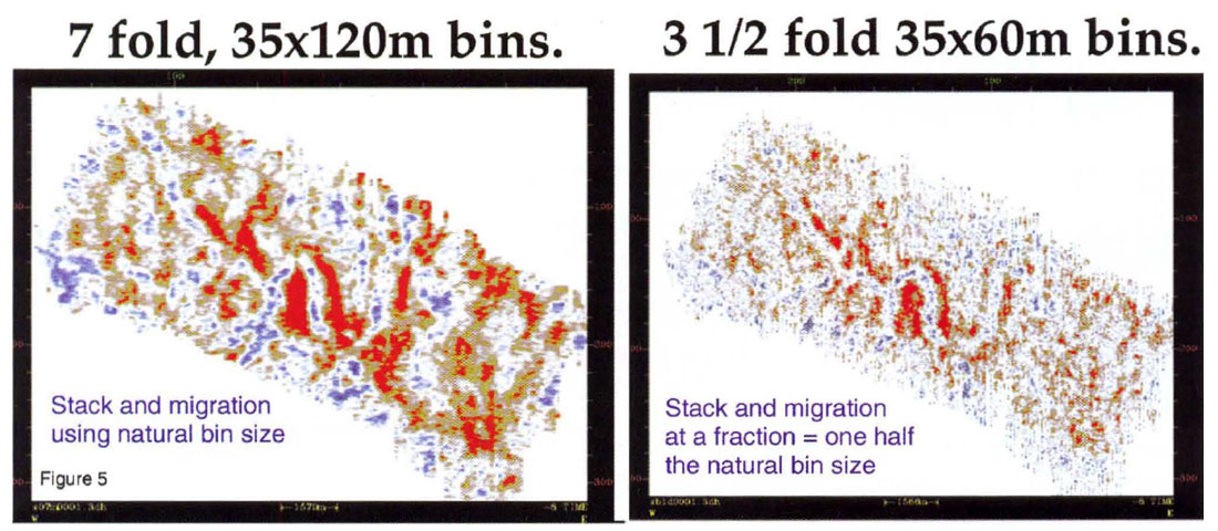
It is also important to test bin size variation. For example, the left side of figure 5. shows one decimation of the 3D survey stacked at natural bin size. The right side of figure 5 shows the same original 3.5 fold decimation, which was stacked at 1/2 of its natural bin size to produce twice as many bins, but half the fold, using the exact same input traces. This test illustrates the importance of bin size choice. Although both processing sequences started with the same surface stations (same number of prestack traces) binning at the natural size for 7 fold yields better S/N but destroys some of the subtle character of the image, such as the smooth shape of the meanders. The failure of the large bins to correctly image the meander is attributed to the intolerance (of post stack finite difference migration) to excessively oblong bins. Modern Kirchoff prestack and poststack algorithms, with careful anti-alias on the operator, have imaged bins up to 4:1 aspect ratio without significant artifacts, (apart from some frequency limiting).
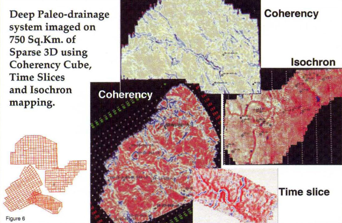
Ultimately these tests illustrated that far less effort and expense was required to illuminate our subsurface targets with 3D seismic, than we had previously expected. Given a low cost exploration tool, Amoco proceeded to acquire several other (large) 3D surveys in the area, totaling more than 750 sq. km. of 10 fold 3D. The quality of this inexpensive Sparse 3D is more than adequate for our targets, as well as other features such as the extensive paleo drainage system shown in figure 6. This example clearly illustrates the importance of the "big Picture" view, as opposed to the high resolution "postage stamp" option.
In 1994 the concept of scaling line spacing to be wider for deeper targets was extended to varying acquisition parameters across a foothills structural 3D survey to reduce cost. The insight here amounts to the recognition that fold should be kept constant with (structured) stratigraphy, and not with depth. This requires fairly tight shot and receiver line spacing over the crests of anticlines, but allows much wider shot and receiver line spacing over the flanks of the structures and even less effort in the syncline areas. The overall effect of this redistribution is that a useful image requires far less effort. The whole effect improves through the use of 3D prestack depth migration, and figure 7. through figure 10. show examples of this.
Prestack depth migration can position output trace images at arbitrarily defined bin center positions, by sampling the migration operator at any output grid position desired. Quality of the final output image is now a function of the interrelated effects of acquisition shot and receiver station spacing, as well as output migrated grid spacing. The effect of reduced surface sampling for structural targets was investigated using prestack depth migration in the same way as the standard processing techniques were used to test reduced acquisition effort on stratigraphic targets.
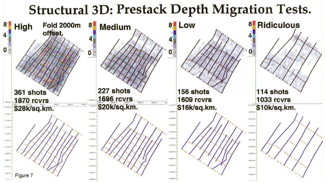
Four trial acquisition configurations are shown in figure 7. The top left of figure 7. illustrates the actual field acquisition and associated cost. The remaining three decimations each reduces surface effort by approximately one half the previous design. (Estimated costs for these trial acquisition schemes are also shown for economic comparison.)
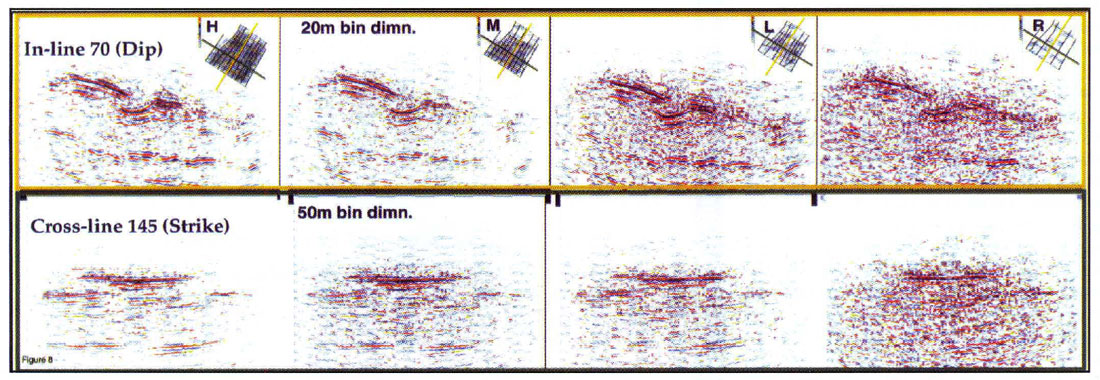
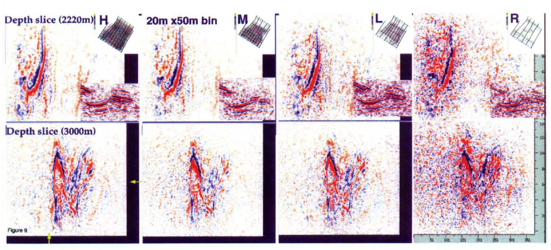
Results of prestack migration on these four decimations are shown in figure 8. and figure 9. The dip and strike sections, shown in figure 8., indicate that the most prominent features of the structure remain visible down to absurdly low levels of surface effort. Generally the reduction in surface spatial sampling tends to increase the noise level, and masks some subtle features, as fold drops. Again these tests help determine what types of subtle seismic features are important for a play, and the required level of surface occupation to image them satisfactorily. The depth slice plots in figure 9. show a similar consistency in general features, with an increase in noise as fold drops. Interestingly the positions of shot lines have unexpected control over resolution. The depth slices on figure 9. show better imaging (on the plunge of the structure on the east) at the lowest and highest fold levels, rather than either of the intermediate decimations. This occurs because the intermediate decimations are missing a critical shot line, which is present in the lowest fold decimation.
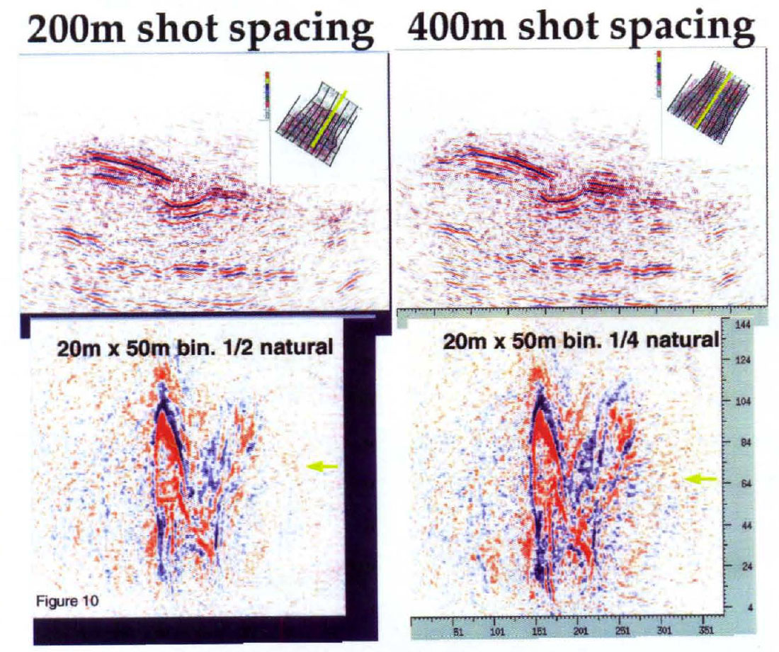
Strictly speaking, while bin size is not an issue for prestack depth migration, surface spacing of shots and receivers will make a difference. Imaging to different sized bins with prestack migration will not yield much of a test (consider each output trace a bin of arbitrarily small area); however, testing different station spacing is a valid comparison. For heliportable work, shots are very expensive, so maximizing the shot station spacing will yield large cost reduction. Migrated images of two shot station spacing is shown in figure 10. Even though the 400m shot spacing decimation used slightly fewer traces the image is comparable with shots spaced at 200m, and although somewhat noisy shows better detail of the structure. This is another indication that randomness in acquisition allows enough scatter in subsurface coverage to successfully migrate 400m shot station data to an output line spacing of 50m without significant migration artifacts.
The fundamental point behind Sparse 3D is: conventional wisdom (and/or fear of failure) has kept many people stuck with the old paradigm that all 3D's need high fold, high resolution parameters, regardless of the target depth. Choosing parameters that are appropriate for our exploration plays allowed us to make extensive use of both foothills heliportable, and conventional 3D's to explore a large number of plays during the last four years.
If we were foolish enough to use traditional high fold, tight line and station spacing parameters, the same surveys would have been four times as expensive, without providing significantly more information about our focused targets. (Although the data would probably look very nice!) Rather than emphasizing that Sparse 3D saved Amoco Canada millions of dollars, it is more realistic to say that Sparse 3D brought the cost of investment down to the level where we could aggressively pursue play concepts far faster. cheaper and better than are otherwise possible, and also to make many more play types economic to chase.
One final sobering note: the 3D survey is pointless if we fail to capture the minimum level of detail for interpretation that leads to economic success. Equally important, (and more insidious) if we continually overdesign 3D survey using theoretical worst case upper limits for spatial sampling. we make the exploration plays less economic, or worse. shoot less 3D, and miss play opportunities entirely.

Acknowledgements
A. Powers, C. Martin, D. Cottle. A. Richards, D. D' Amico, D. Terne , T. Zwicker, G. Cain. T. Dickson, D. Au, S. Gray, J. Etgen, C. Regone and J. Smith.


Join the Conversation
Interested in starting, or contributing to a conversation about an article or issue of the RECORDER? Join our CSEG LinkedIn Group.
Share This Article