Sparsity and band-limitation: Two sides of the same coin?

We introduce a strategy to identify the optimal sampling functions for Fourier reconstruction (5D interpolation) methods. We integrate the concepts of band-limitation and sparsity into a single decision criterion to select the sampling functions with the least amount of spectral interference in the Fourier domain. The analysis was carried out for two-dimensional (2D) random and regular sampling functions. It is possible to find regular sampling functions, in addition to random sampling functions, that are optimal to reconstruct the signals with sparse Fourier spectral support. However, regular sampling scenarios outperform random sampling functions for band-limited spectral supports.

Introduction

The performance of Fourier reconstruction methods is highly dependent on the type of sampling function (Naghizadeh and Sacchi, 2010). Sampling functions can be classified into two categories, uniform and non-uniform. In uniform sampling methods, a signal is sampled periodically at a constant rate. This leads to recovery conditions based on the well-known Nyquist sampling theorem (Unser, 2000). Traditionally, in the signal processing community uniform sampling was preferred to non-uniform sampling. However, in recent years, with the introduction of Compressive Sensing (CS) methods, the attention has shifted toward non-uniform sampling (Donoho, 2006). The CS concept facilitates the robust reconstruction of a signal using a specific basis such as Fourier coefficients.

Fourier reconstruction methods rely on two basic assumptions. In general, we assume signals are either band-limited or sparse in the wave-number domain. Examples of the aforementioned assumptions abound in the signal and image processing literature. In the geophysical literature Duijndam et al. (1999) and Schonewille et al. (2003) proposed a band-limited signal reconstruction method for seismic data that depends on two and three spatial dimensions. Methods that use the sparsity assumption to reconstruct seismic data were proposed by Sacchi and Ulrych (1996) and Sacchi et al. (1998) and expanded to multidimensional data by Zwartjes and Gisolf (2006), Zwartjes and Sacchi (2007), and Trad (2009). The sparsity principle has also been used for the purpose of seismic bandwidth extension (van Riel and Berkhout, 1985). Generally speaking, the sparse signals can also be considered as band-limited signals, but with arbitrary support regions in the Fourier domain.

In this article we aim to find a measure for identifying the optimal sampling functions for Fourier reconstruction methods. We fuse the concept of band-limitation and sparsity into a single framework. This paves the ground for developing a fair selection criteria between regular (uniform) and random (non-uniform) sampling functions. Therefore, the sampling function with the least amount of spectral interference is identified as the optimal sampling scenario. The proposed strategy is tested on various two-dimensional sampling functions.

Methodology

We analyze Fourier reconstruction potentials for four regular and one random two-dimensional (2D) spatial sampling scenarios (Figure 1). We create a sampling grid of 16x16 samples on which the filled circles (values equal to 1) show the available samples and empty circles (values equal to 0) represent the missing samples. Figure 1a shows the full sampling operator. A fully sampled grid will have a simple spike representation at the middle of its Fourier representation (Figure 2a). For 2D Fourier spectrum plots in this article (Figures 2-7), we use normalized wave-number notation. This means we assume the distance between the spatial samples to be one. The exact wave-numbers can be obtained by dividing the normalized wave-numbers (kx and ky) by the actual spatial sampling interval in X and Y directions, respectively.

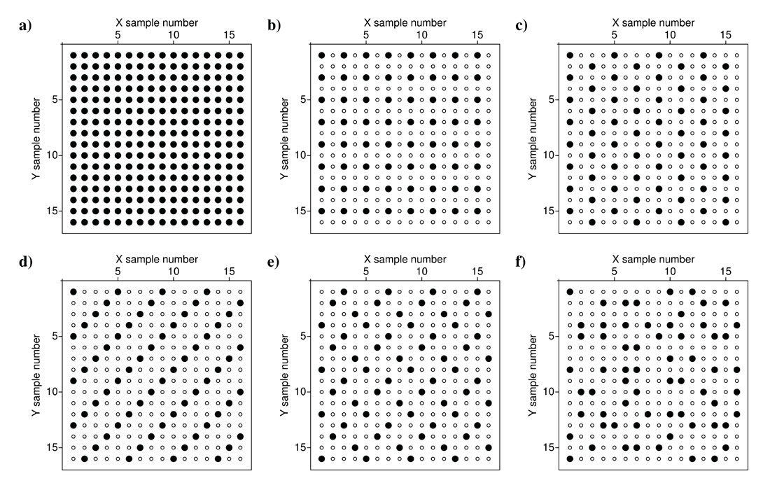
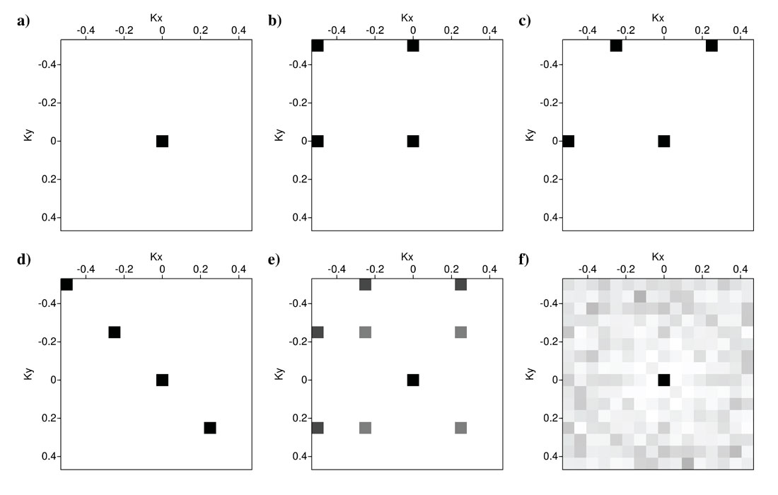
Introducing missing samples (empty circles) to the spatial grids (Figures 1b-1f), results in emergence of new spikes in the Fourier domain responses of sampling operators (Figures 2b-2f). The size and location of these spikes will depend on the type of spatial sampling function. Throughout this paper darker colors in spectral plots will represent higher amplitudes. Figures 1b, 1c, and 1d show 3 different scenarios of regular sampling operators with 75% missing traces. Figures 2b, 2c, and 2d show the Fourier responses of the sampling operators in Figures 1b, 1c, and 1d, respectively. These 3 Fourier responses have 3 new spikes in addition to their original spike at (kx, ky)=(0,0). Notice that all of the spikes in Figures 1b, 1c, and 1d have equal amplitudes. Figure 1e shows another regular sampling scenario with 75% missing samples. This sampling operator is derived from the regular sampling operator in Figure 1d by applying 90 degree rotation to every other pair of neighboring available samples. Figure 2e shows the Fourier response of the sampling operator in Figure 1e. The Fourier response of this regular sampling operator has 8 new spikes but all of them have smaller amplitude than the original spike at (kx, ky)=(0,0). Finally, Figure 1f shows a random sampling scenario with 75% missing samples. Figure 2f shows the Fourier response of the sampling operator in Figure 1f. Random sampling introduces spikes all over the Fourier domain but the amplitude of these spike are very small compared to the original spike at the origin. This is an important property of random sampling as it prepares the ground for sparse Fourier recovery of data.

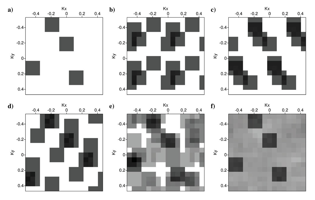
We create a synthetic sparse Fourier signal shown in Figure 3a to investigate the principles of Fourier data reconstruction. We have 4 squared areas (grey squares) which contain desired signal (complex number with amplitudes equal to one) and the rest of the Fourier domain is zero. It is not important what the signal looks like in the spatial domain as primary concern is that our Fourier representation is sparse. Of course, for the fully sampled data (Figure 1a) the Fourier representation of the signal would be the original spectrum (Figure 3a). Sampling the signal in the spatial domain (point by point multiplication of sampling operators (Figure 1) with original data samples) is equivalent to circular convolution of Fourier responses (Figures 2a-2f) with the original spectrum (Figure 3a). Therefore, by sampling our signal in the spatial domain using the sampling operators in Figures 1b-1f we obtain the Fourier spectra of the sampled signals in Figures 3b-3f, respectively. The aim of Fourier reconstruction is to recover the original spectrum (Figure 3a) using the spectra of sampled data (Figures 3b-3f) and their correspondent sampling operators (Figures 1b-1f). The Fourier reconstruction works best for the Fourier sampling responses which have low amplitude spikes everywhere except at the origin (kx, ky)=(0,0). One can easily detect with the naked eye that the random sampling scenario (Figure 3f) is the best option for sparse Fourier reconstruction. Among the four regular sampling examples (Figures 3b-3e), only in the Fourier spectrum in Figure 3e the original spectrum is distinguishable from the artifacts introduced by sampling.

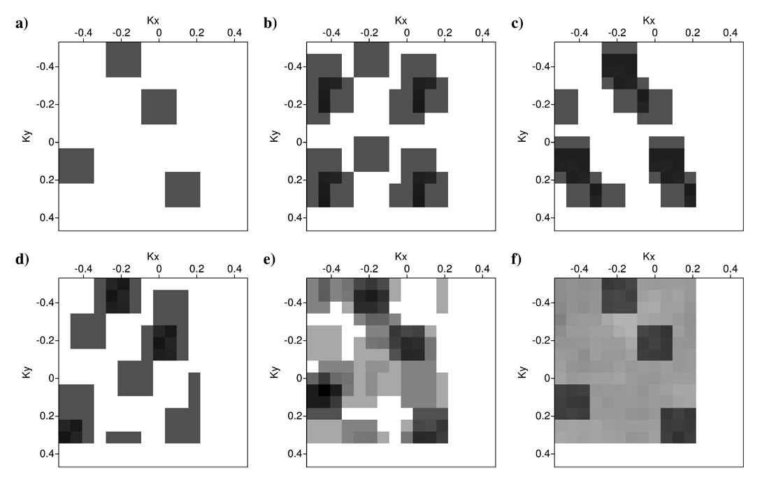
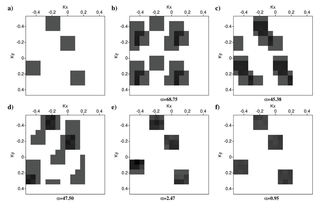
We aim to quantify the success rate for the Fourier reconstruction using a two step algorithm to clean up unwanted Fourier artifacts (Fourier coefficients that are not coinciding with the original Fourier coefficients in Figure 3a). The first step is to use any possible bandlimitation information. This a-priori band-limitation information can be very useful since we can erase any Fourier coefficients that are outside the range of our interest. Let’s assume that we knew beforehand that there was no signal at the normalized wave-number ranges of kx>0.25 and ky>0.3 (this kind of information can be inferred from maximum slope in different directions of seismic events). By deploying the band-limitation criterion, the Fourier representations of sampled data in Figures 3b-3f are reduced to the ones in Figures 4b-4f. The next step is to impose a sparsity thresholding criterion. We can pick a threshold value as the highest value of Fourier coefficients that we want to keep and eliminate the remaining low amplitude Fourier coefficients. For our examples we set our threshold value to be equal to 15% sparse Fourier representation, namely, just preserving the top 15% highest amplitude Fourier coefficients. By imposing the Fourier sparsity criterion on Figures 4b-4f, we obtain the Fourier representations in Figures 5b-5f. We can calculate a difference value of α for each sampling scenario by subtracting Figures 5b-5f (recovered Fourier spectra) from Figure 5a (the original Fourier spectrum). The difference value (α) for each sampling scenario is written under Figures 5b-5f. Smaller values of α are equivalent to better Fourier reconstruction results. The random sampling scenario (Figure 5f) with α=0.95 leads to best Fourier reconstruction. Three of the regular sampling scenarios (Figures 5b-5d) with α=68.75, α=45.38, and α=47.50 are the worst candidates for sparse Fourier reconstruction. However, the regular sampling in Figure 1e with α=2.47 (Figure 5e) has a very low difference value compared to the other three regular sampling operators (Figures 1b-1d). This means we can utilize sparse Fourier reconstruction to recover missing samples for this regular sampling operator. However, the random sampling operator remains the best option to reconstruction of missing samples using sparse Fourier reconstruction.

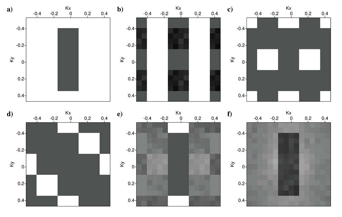
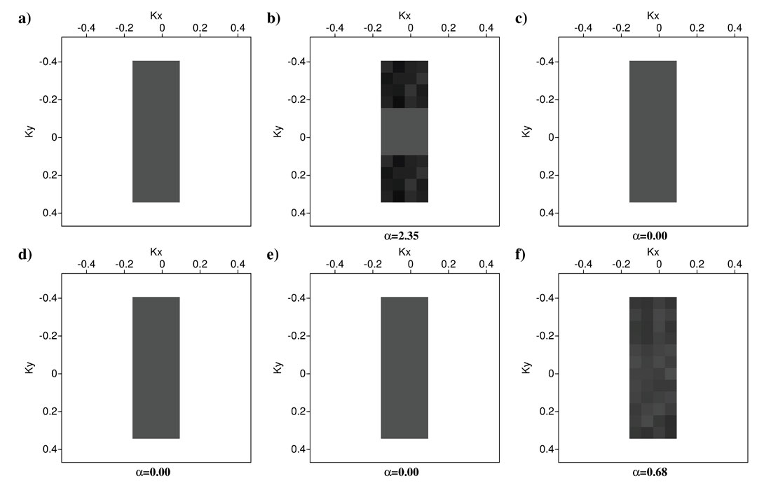
Now we investigate another synthetic data example with a band-limited original Fourier spectrum. For this example we created a band-limited original Fourier spectrum at ranges -0.15 < kx < 0.15 and -0.35 < ky < 0.35 (Figure 6a). Figures 6b-6f show the Fourier representation of sampled signals corresponding to the sampling operators in Figures 1b-1f. In order to implement a band-limited Fourier reconstruction, we preserve the spectral values at the range -0.15 < kx < 0.15 and -0.35 < ky < 0.35 and eliminate the remaining Fourier coefficients. Figures 7b-7f show the band-limited spectra of sampled spectra in Figures 6b-6f. The difference value between the original spectrum (Figure 7a) and the reconstructed Fourier spectra (Figures 7b-7f) is shown under each plot. Three regular sampling operators (Figures 7c-7e) have the difference values equal to zero (α=0). The zero interference between original spectrum and sampling artifacts means we can achieve perfect Fourier reconstruction results. However, one of the regular sampling operators (Figure 1b) has a very high difference value of α=2.35. Also the random sampling operator (Figure 1f) with α=0.68 cannot be favored over three regular sampling operators with α=0. This means that while the random sampling is not the worst sampling method for this synthetic data it is not necessarily the best either.

We arrive at tantalizing conclusions by looking simultaneously at the two above synthetic examples (Figures 5 and 7). First, random sampling operator (Figure 1f) is the best scenario for Fourier reconstruction of sparse spectra with no band-limitations (Figure 5f). However, we might be able to design specific regular sampling scenarios (e.g. Figure 1e) that are suitable for sparse Fourier reconstruction (Figure 5e). Second, regular sampling operators can reconstruct exact Fourier spectrum of desired data if the original spectrum was band-limited (Figures 7c-7e). However, the regular sampling operators must be designed according to the band-limitation information in each spatial direction. Hence, we might be able to find regular sampling scenarios on which both sparse and band-limited spectra can be reconstructed using Fourier reconstruction methods (Figures 5e and 7e).

Conclusions

We introduced an approach for measuring the spectral interferences produced by sampling functions. The proposed strategy integrates the band-limitation information with the sparsity (compressive sensing) principle to find the optimal sampling scenarios. For sparse signals with randomly distributed spectral support the random sampling shows the least interference. However, the regular sampling scenarios show to be the optimal sampling operators for the band-limited spectra. We realized that specific types of regular sampling functions can be used effectively for Fourier recovery of either band-limited or sparse spectra if the signal has more than one spatial dimension. The generalization of proposed strategy to more than two spatial dimensions is straightforward. In fact, adding more spatial dimensions will increase the possibilities for designing regular sampling scenarios with very low amplitude Fourier responses.

For 5D interpolation methods, we can model various combinations of 4D spatial sampling scenarios and select the 4D Fourier spectral responses with the least Fourier artifacts. The results of these analyses can also be used to design 3D seismic surveys that are best fitted to be regularized using 5D interpolation methods. Using a combination of regular and random sampling operators along different spatial dimensions for a 3D survey might prove to be optimal for 5D interpolation methods. As a general rule of thumb, it would be desirable to use random/regular sampling operators along the dimensions with sparse/band-limited wave-number representations, respectively.

Acknowledgements

This research was funded by the generous support of the industrial members of the Signal Analysis and Imaging Group (SAIG) at the University of Alberta.