Squeezing more from seismic data: Application of prestack simultaneous impedance inversion to a stratigraphic and structurally complex productive field in Argentina

The need to revitalize conventional productive old fields led the geology and geophysics groups to consider the implementation of accurate methodologies and analysis for arriving at static geomodels. An example at hand is the Golfo San Jorge Basin in Argentina with the complexity of its productive zones. Careful reprocessing of seismic data was carried out followed by correlation with well ties and followed by prestack simultaneous impedance inversion. As a result, several zones with distinctive characteristics were identified, one which had been drilled with remarkable success compared with the historical results in that sector of the basin. This led to an encouraging decision by management to continue prospecting for new opportunities, which led to more drilling with exciting results. The careful evaluation of the data and the methodology adopted has significantly contributed to the development of the field.

Introduction

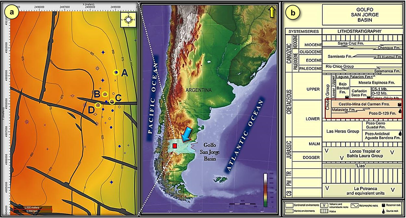
During the evaluation of an oil and gas productive area located on the west flank of the Golfo San Jorge Basin, Argentina (Figure 1), it was proposed that the available seismic data be reprocessed. The reprocessing exercise was expected to include prestack time migration, enhanced frequency content and thus resolution, and more importantly, amplitude preservation. The reprocessed seismic data was put through prestack simultaneous impedance inversion to obtain P- and S-impedance attributes, and hence VP/VS ratio. These attributes were then used to interpret lithology, porosity and fluid saturation in the target interval, and helped minimize risk during the planning and drilling of new wells.

Geological context

The area of study is located in Golfo San Jorge Basin, Argentina. It is a continental rift basin broadly east-west oriented, and located in the extra-Andean Patagonia, between 45° and 47° S latitude (Figure 1). It was developed under a discontinuous extensional regime from the Late Jurassic to Middle Miocene showing several phases of normal fault reactivation (Paredes et al., 2013). During the Late Cretaceous and the Cenozoic, the basin developed as a wide depositional area with low tectonic subsidence, where accommodation was generated mainly by sea-level fluctuations and extensional tectonics in a passive margin setting. The westernmost part of the basin, close to the Andean Cordillera, was subject to positive tectonic inversion along the San Bernardo Fold Belt. This geological setting is ideal to study fault kinematics and growth fault mechanisms because previous studies have identified two fault sets with different dominant strikes coming out of a single rift event with changing extension direction or two different rift events.

It is interesting to keep in mind that the Cretaceous Chubut Group provides up to 47% of the liquid hydrocarbons of Argentina, obtained mainly from fluvial channel belts of the Cañadón Seco (Bajo Barreal) Formation. Faults are a key component of many hydrocarbon plays, and their growth, linking and overall evolution impact on the coeval topography, sediment routes and distribution of clastic facies. Additionally, the approaching, interaction and the timing of ramp relays breaching are critical to predict the occurrence of sub-seismic sandstone reservoirs in hanging-wall fault blocks. Furthermore, complex linkages between shallow and deep fault systems associated with different extensional phases have significant control on the hydrocarbon preservation (Paredes et al., 2018).

The Pozo D-129 Formation (Barremian-Aptian) mainly of lacustrine origin, with moderate organic content, is the most important source rock in the basin, and is producing in some places. Overlying it is a group of fluvial- shallow lacustrine units deposited under late sag conditions that contain the reservoirs. During the Tertiary, an alternation of marine and continental deposits took place as well as the compressional uplifts of the N-S trending San Bernardo fold belt through the reactivation of some previous normal faults. The Quaternary deposits, very widespread over the whole Patagonia, represent drastic climatic changes, such as glaciations, and the consequent sea level fall. After migrating through a network of faults and pathways, the oil is trapped in both extensional and compressional structures (Sylwan, 2001 and Sylwan et al., 2008).

Seismic data reprocessing

Seismic impedance inversion assumes a stationary wavelet and amplitude preservation, along with the underlying assumption that the seismic data mimic the subsurface geology and contain very little noise. It is also important that the seismic reflection events are all primaries and contain no multiples. In addition to this, the bandwidth of the seismic data affects the inversion results in two ways: 1) the lack of higher frequencies in the seismic data prevent resolution of thin layers in the zone of interest, and 2) the absence of lower frequencies prevent the incorporation of the basic impedance structure of the earth model that is being arrived at. Our seismic data was first acquired and processed in 2001 and processed again in 2008.

With the above assumptions and observations in mind, in 2017 it was decided to reprocess the seismic data and ensure amplitude preservation as well as attempt to improve the frequency content. The preliminary processing sequence included bad trace editing, spherical divergence correction, shot-related noise attenuation, surface-consistent amplitude compensation and deconvolution. Tomographic reflection statics were estimated and applied; velocity picking, surface consistent residual statics and 5D interpolation also formed part of the processing flow. Quality control for amplitude preservation was carried out at each step.

An initial post-stack Kirchhoff migration was first carried out against which the subsequent prestack migrated data could be compared with. Next, two iterations of RMS velocity updates through residual moveout picking yielded the final RMS velocity field which was used for running the Kirchhoff migration with straight ray approximation. This was followed by another pass of RMS velocities which was then used for interval velocity estimation using constrained Dix inversion (Dix, 1955). A final pass of Kirchhoff migration with curved ray approximation (Yilmaz, 2001) generated the final seismic data volume.

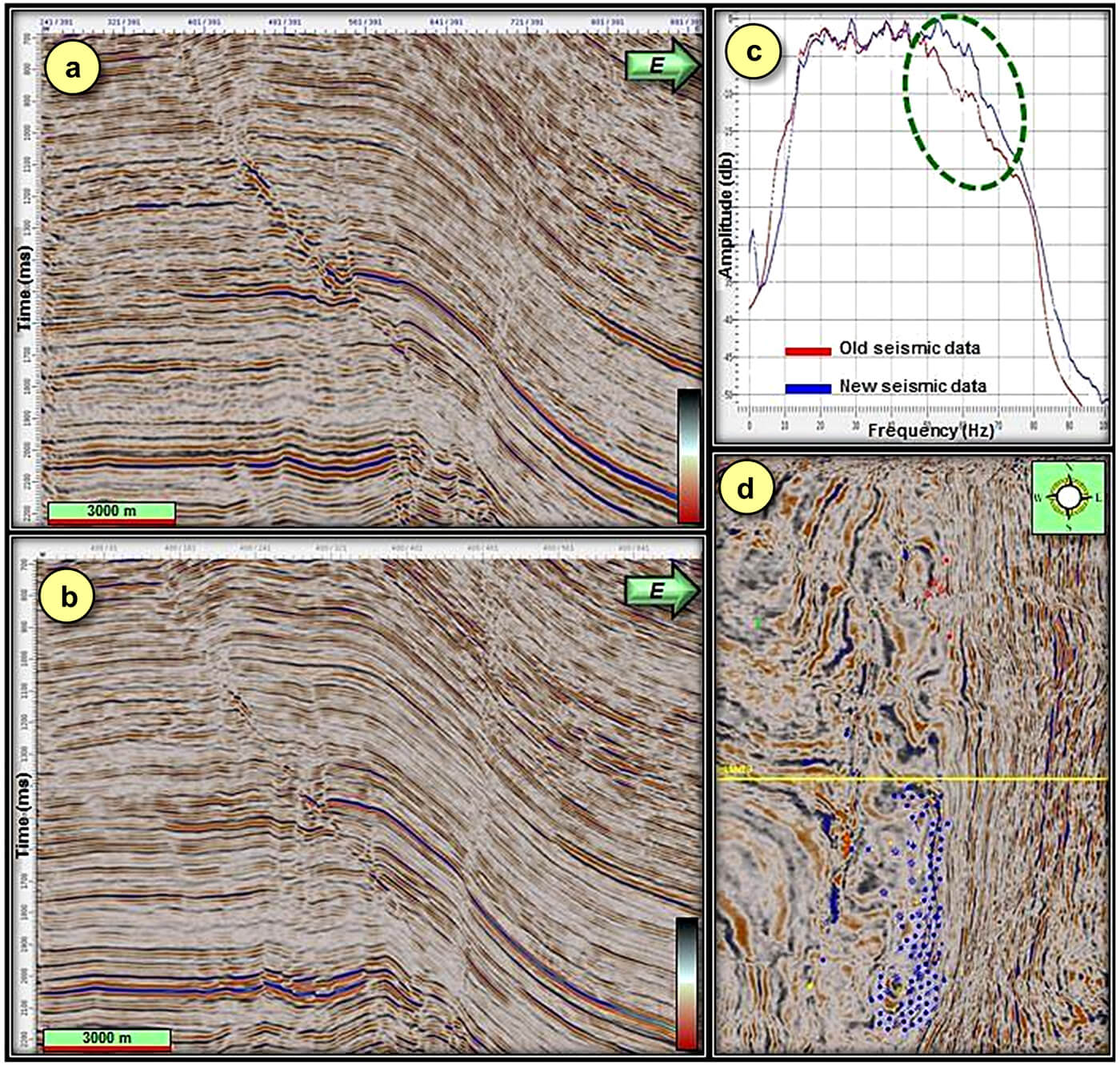
In Figure 2, a crossline section is shown from the old vintage of the seismic data (Figure 2 a) and the equivalent section from the reprocessed version (Figure 2 b). The frequency spectra for both cases are shown in Figure 2 c. Not only do we see an enhancement in the frequency content of the reprocessed data, the imaging of the faults is also crispier. A time slice from the 3D seismic volume is shown in Figure 2 d, wherein the yellow line shows the location of the crossline shown in Figure 2 a and b.

Interpretation of seismic data

Satisfied with the improvements seen in the reprocessed seismic data, the next step was to redo the interpretation. This exercise started with correlation of well log data with the seismic in terms of linking the main geological markers with their corresponding seismic reflections. This yielded an initial framework for drawing up a probable geological model for the subsurface in the area of interest.

Figure 3 a shows a west to east seismic section, depicting the complexity of the subsurface in the study area. The main overthrust and associated faults are seen as the clear architectural elements of the structure and are indicative of how the stratigraphy got affected over the different tectonic stages. We attempted to highlight the seismo-geological characteristics in the data in terms of fault zones, their limits and terminations, etc. by using the high-frequency Amplitude Volume Technique (AVThf; Vernengo et al., 2017).

Figure 3 b exhibits a west-to-east seismic section extracted from the AVThf volume. The display helps illustrate the various kinds of reflector geometries together with their faulting.

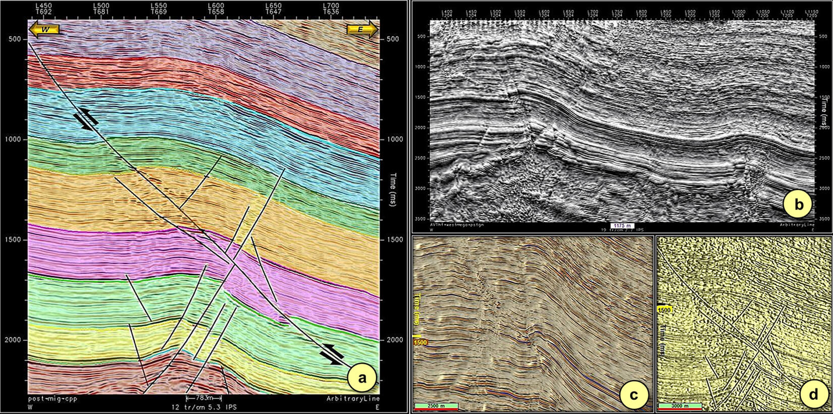
The advances in image processing techniques allow determining some characteristics when they are used in seismic plots that can be used to recognize patterns. One of these image attributes is apparent roughness which is determined using a color frequency filter. This process of images can sometimes help interpreters to visualize rubrics observed with consistency and continuity. Thus, surface roughness displays exhibit some uneven patches or sequences of shorter cycles and others at somewhat longer cycles, which help decipher signature patterns on the images.

The blocked seismic appearance attribute display is the reconstruction of the input image as partitioned square blocks of very small size (few pixel squares) and help with interpretation of fine discontinuities along block boundaries. Both the roughness and blocked visual seismic attributes can be generated using workstation software (AUTOCAD) and can form an important step in the seismic interpretation workflow, especially in cases of complex subsurface structures. Visual examination of the data through AVThf displays and through the roughness and blocked image attribute (Figure 3 c and 3 d) helped arrive at a more accurate static model of the subsurface.

Case study

The area of study is over an oil and gas field located in the Golfo San Jorge Basin in Argentina (Figure 1) and has been exploited since the 1960´s. Over 90 wells have been drilled in the field and the daily production is 650 barrels of oil and 280,000 cu. ft. of gas. The seismic data used for reservoir characterization cover an area of 160 sq. km., with six interpreted horizons and various interpreted faults. Four key wells have been selected for use in this study, based on their production history and strategic location in the field. The time window selected for impedance inversion was 800 ms thick, and covered part of the traditionally productive and prospective reservoirs (Pozo D129 Formation in Figure 1).

Rock physics analysis

The characteristics of the reservoirs being studied included the presence and thickness of tuffaceous sandstones, and the uncertainty in the salinity of the formation water. These conditions made the definition of lithofacies in the target zones a challenge for seismic impedance inversion. Thus, before going ahead with prestack simultaneous impedance inversion, it was advisable to analyze the rock physics properties using the available well log data. For doing so, the well log curves for four key wells (A, B, C and D, Figure 1 a over the 3D seismic volume were selected up and edited for washout zones as indicated on the caliper curves. Different elastic properties were then derived from the basic log curves (VP, VS and density), as well as the petrophysical properties such as lithology, water saturation and porosity. Such properties were next analyzed by way of crossplotting to determine reliable relationships between them which could then be used to calibrate to seismic data, considering their vertical resolution (see Figure 4).

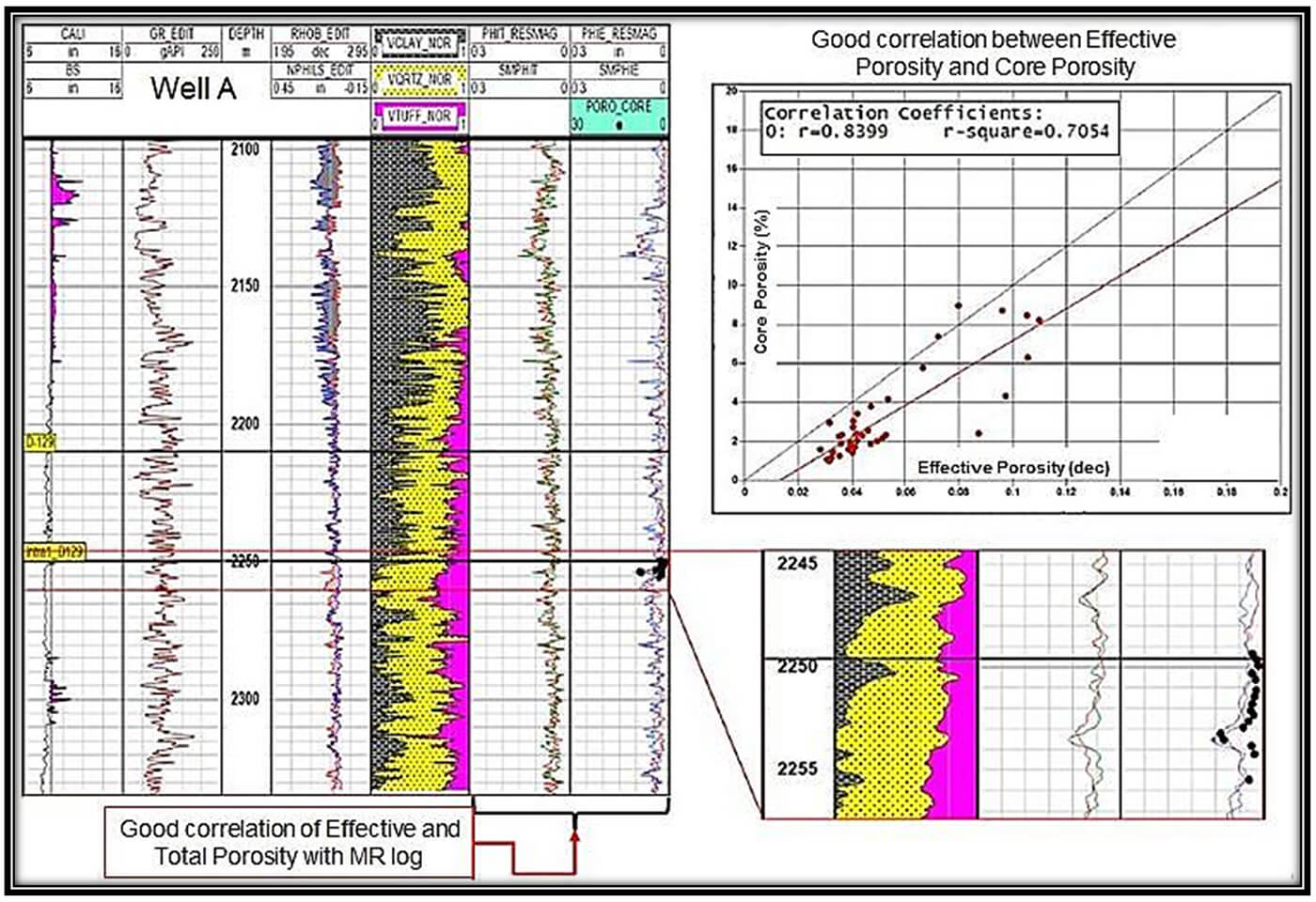
Fortunately, valuable information such as production data, the total gas curve, lithological descriptions and porosity, plugs and a couple of cores were available, which could be used for calibration of the petrophysical model derived from well log data.

Using the caliper, gamma ray, resistivity and density curves for the four key wells, other curves were derived such as volume of clay, quartz and tuff, porosity, water saturation, gas content and lithology. Cut off values used in the well-log interpretation were carefully selected.

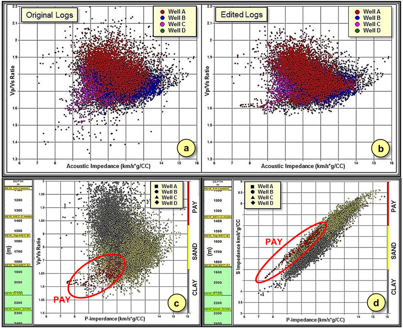
The correlation between the porosity calculated from a conventional analysis, and the porosity calculated by way of NMR (nuclear magnetic resonance) log curves was obtained. The analyzed core porosity values show the same trend that the effective porosity curves in different depth intervals. Figure 5 a shows a comparison of crossplots between the acoustic impedance versus VP/VS for log data from four key wells before and after the data were edited. The editing removed the outliers but preserved the overall trend of the cluster points.

Again, using the data from the four key wells, cross-plots between P-impedance and VP/VS in the indicated depth intervals therein is shown color-coded with lithology is shown in Figure 5 b. Although an overlap between the three lithologies is seen on the cluster plots, the points corresponding to the clay zone can be seen separated from those from sand and pay zones. Similarly, the crossplot between P- and S- impedance shown in Figure 5 c and d exhibits a somewhat different alignment of the points corresponding to clay, sand and pay zones.

Seismic impedance inversion

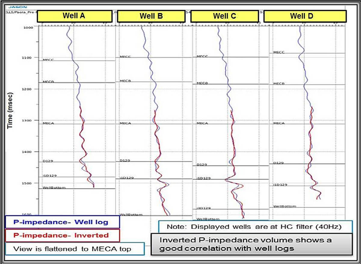
To understand the target subsurface formations better, we turned to prestack simultaneous impedance inversion. The derived elastic properties will be used to study the distribution of porosity as well as determination of reservoir pay zones. The impedance inversion was carried out between the two markers, namely MEC A (Mina El Carmen Formation bottom) and intra 3_Pozo D 129 Formation (see Figures 6, 7 a and 7 b).

The complete exercise was carried out in four steps comprising the conditioning of seismic data, deriving low-frequency trend volumes, the facies and probability analysis and finally the porosity estimation.

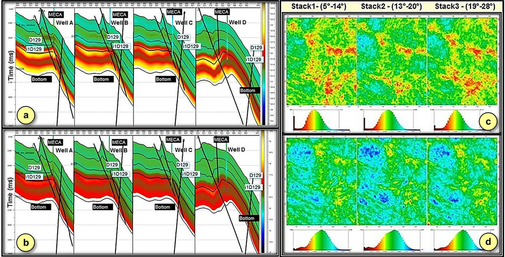
As the first step, an initial pass at noise reduction was used to improve the signal-to-noise ratio. Three angle stacks (with angle ranges 5°-14°, 13°-20° and 19°-28°) were then generated for use in simultaneous inversion. Signal-to-noise ratio maps were generated as part of the quality control before and after conditioning as shown in Figure 7 c and d, which validated the application of the noise removal process.

In this case the abbreviated sequence applied for gathers conditioning was: dense residual moveout analysis and correction (up to 30 deg incidence angle), dense fourth order residual moveout analysis and correction (high incidence angles), trim statics and correction, spectral whitening, footprint analysis and compensation, cross offset amplitude analysis and compensation, stretching modeling and compensation, residual random and organized noise attenuation (Radon filters/Median filters) and angle mute.

Next, well to seismic ties were carried out for the four wells available over the 3D seismic volume. The well reflection coefficient series were then compared with the seismic traces at their respective locations to estimate the wavelets. An average of these wavelets was then used in the impedance inversion process.

To add the low-frequency background trend, the seismic interval velocity volume obtained from processing and calibrated to local well velocities (sonic and VSP) was used. This low frequency velocity model was horizontally constrained with the interpreted horizons.

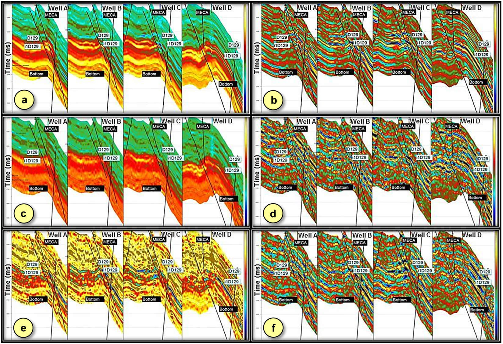
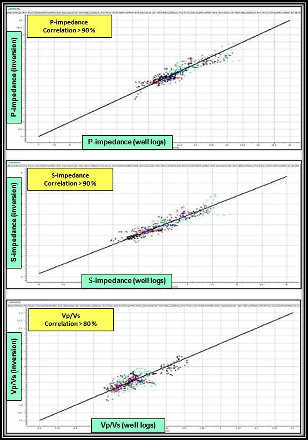
Simultaneous impedance inversion was then carried out on the data to obtain P-impedance and S-impedance volumes (see Figure 8). Both these volumes were used to compute VP/VS ratios. The measured P-impedance at the different well locations was crossplotted with the inverted P-impedance at those locations. The strong linear correlation observed on the plot lends support to the inversion process. Equivalent crossplots were generated for S-impedance and VP/VS ratio, again with similar results (see Figure 9).

Within our broad zone of interest, we constructed crossplots between different pairs of rock physics parameters (P-, S-impedance, VP/VS, Lambda-rho, Mu-rho, etc.) from well log data, and then crossplotted the same parameters derived from seismic data. Favorable correlations were noticed between them (see Figure 10). Next, we associated geologic facies (pay, sand, clay) interpreted on well log data within the intervals with the clusters on these cross-plots, to estimate the distribution of lithofacies. The relative proportion of each lithofacies in the zone of interest was then estimated which allowed us to generate the weighting factors (Figure 11) used in the next step.

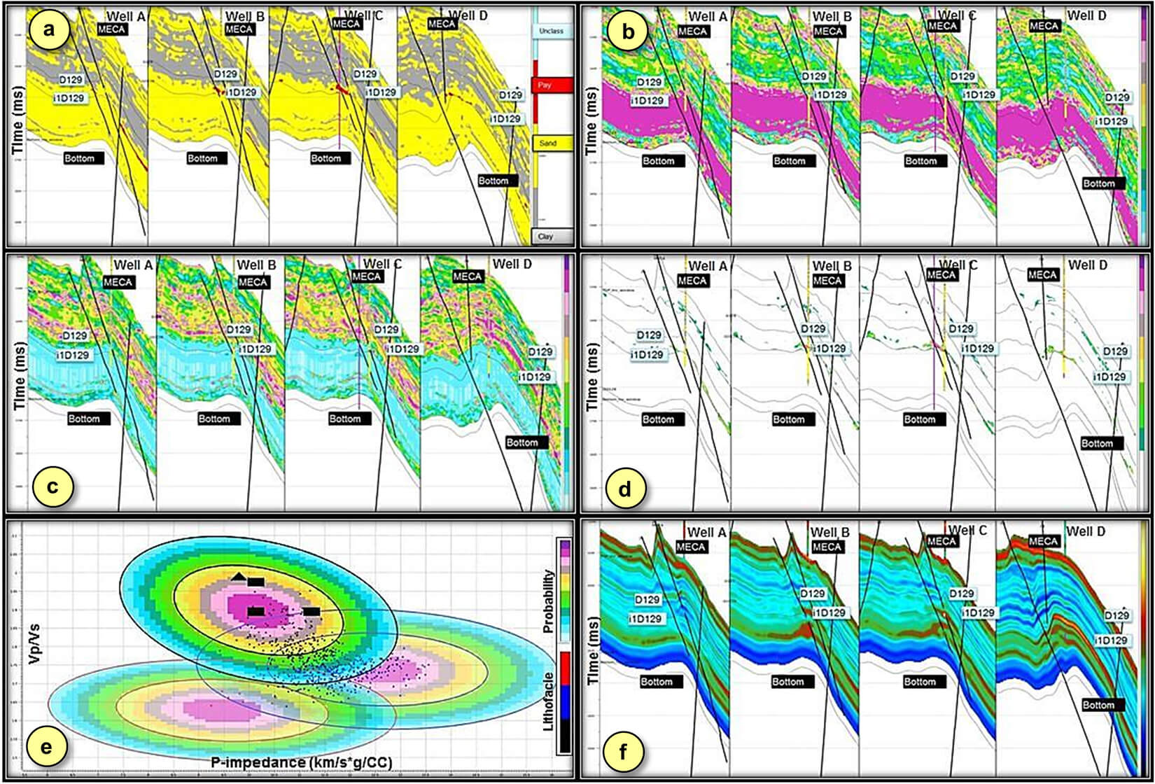
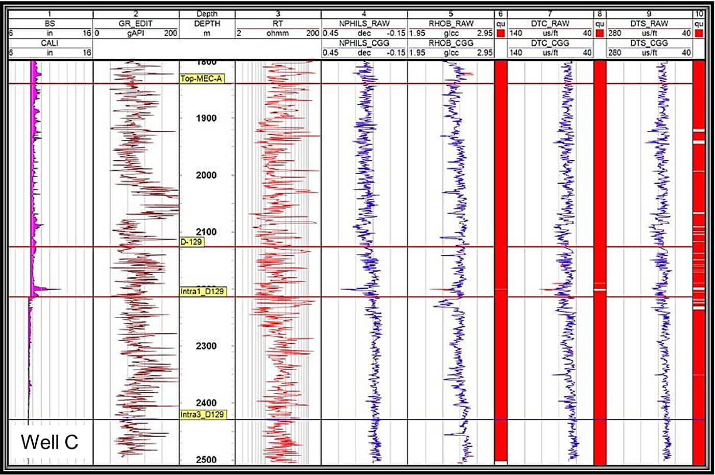
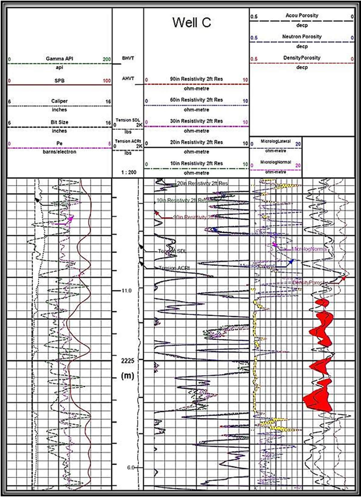
In Figure 12 it is possible to appreciate the logs from Well C in the vertical zone of the gas reservoir highlighted in red color. Once this step was carried out to our satisfaction, the probability density functions were defined on the crossplots for each lithology including the litho-weights determined in the previous step. It was defined three polygons for the main recognized facies. The points near the center of each polygon have more probabilities to represent that facies than the rest of the points inside the same polygon. This approach allowed us to account for the uncertainties associated for each facies. Such work follows the Bayesian classification approach and provides a facies model reflecting the quality of the litho-units and its associated uncertainty analysis.

The first drilling results

In Figure 13 a and 13 b we show a stratigraphic slice at the level of interest from the P-impedance and S-impedance volumes. Well C is the new well drilled and exhibits a low impedance anomaly. The west-to-east sections from the derived ‘probability of pay’ volume and the ‘effective porosity’ volume are shown in Figures 13 c and 13 d respectively. The green log curve is the resistivity curve and the red curve the spontaneous potential curve. The yellow arrows indicate the main gas productive zone.

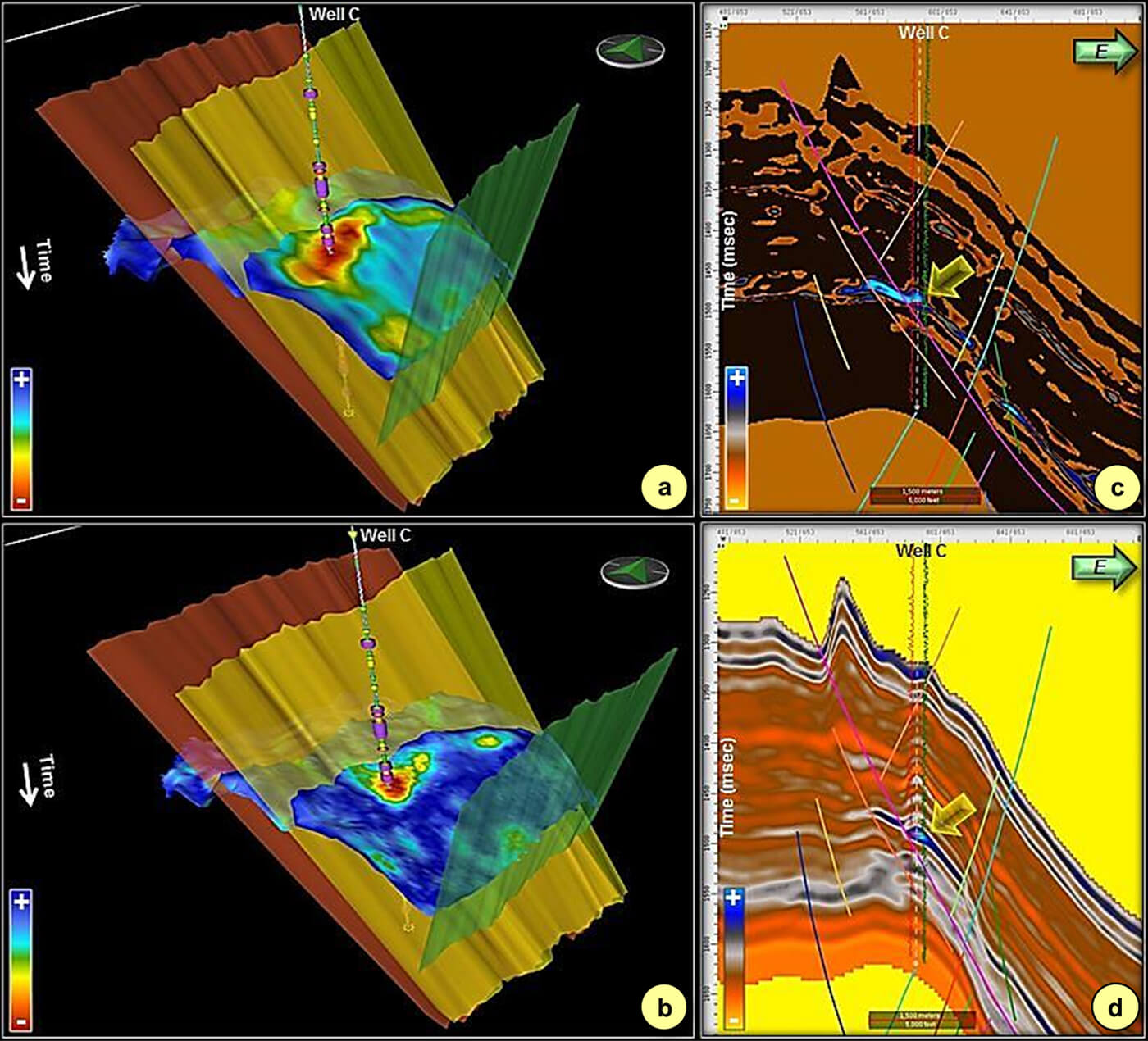
In Figure 14 we show the extracted geobodies corresponding to low impedance values, which correlate with the other petrophysical attributes volumes mentioned above. Per the results of the impedance inversion exercise and the ensuing analysis, three wells were drilled at different locations on the 3D volume, but through the low-impedance anomaly which corresponds with high values for porosity and probability of pay (see Figure14).

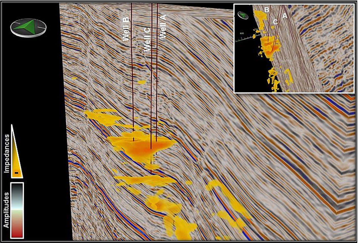
As per the initial production tests (without fracking), Well C flowed gas (10,030,000 CFD, computational fluid dynamics) through a 12 mm choke, with a dynamic pressure of 2,100 psi and a static pressure of 2,800 psi. Well B drilled to the west of Well C, after fracking flowing gas (1,406,000 CFD). Well A drilled over the border zone of the main recognized geobody seen in Figure 14, produced very little gas (1,060 CFD).

Conclusions

The reprocessed seismic data exhibited good quality in terms of better resolution as well as multiples attenuation and showed reasonably good correlation with well data.

Facies and fluid probabilities captured most of the known pay zones based on the lithotype log. High probability of pay correspond to low impedance and low VP/VS ratio. Based on the results of this exercise, three wells were drilled, two of which were good wells and the third one as per our expectation.

In this study the place to drill up to Fm. D-129 from the Seismic Inversion interpretation results. This give confidence to determine the final location because previous wells, did not were profitable because bad reservoir conditions.

The approach followed in this study has certainly increased the probability of success in the area and has encouraged us to apply it to other company assets.

Acknowledgements

We sincerely thank Satinder Chopra, from TGS Canada, who painstakingly rewrote many parts of this paper. We also thank Juan Moirano, Javier Scasso, Ignacio Rovira and CGG GeoSoftware team for their contribution to this paper. Finally, we thank Pan American Energy for permission to show the examples in this article.