Stochastic Seismic Inversion Applied to Reservoir Characterization

Seismic inversion has been used for several decades in the petroleum industry, both for exploration and production purposes. During this time, seismic inversion methods have progressed from the initial recursive inversion method to the present plethora of methods and software packages available to transform band-limited seismic traces to impedance traces. The application of seismic impedance data has also progressed from qualitative assessments of prospects to the quantitative description of reservoir properties necessary for reservoir characterization.

Reservoir characterization requires the construction of detailed 3D petrophysical property models contained within a geological framework. Structural interpretation of seismic data has been and continues to be important in the generation of the framework of the reservoir model. Seismic data has been less frequently involved in the generation of the petrophysical parameters that populate the 3D model. There are several reasons for this lack of application of seismic data to property modeling - lack of a 3D dataset (only 2D data available), inability to relate seismic data quantitatively to reservoir properties, and lack of sufficient vertical resolution to generate detailed property models. The pervasive availability and acceptance of 3D data has substantially overcome the first obstacle. Seismic impedance volumes calculated from these 3D datasets can, for many reservoirs, provide a seismic parameter that can be directly related to a reservoir property (porosity, for example), thereby addressing the second problem. The last problem - the lack of sufficient vertical resolution for characterization applications, has been a more difficult problem to solve. Stochastic seismic inversion is one method that can provide the vertical resolution sufficient to generate detailed 3D reservoir property models.

Seismic resolution is a function of the frequency of the recorded seismic wavefield and the velocity of the medium. Although some enhanced recovery methods, such as steam floods or fire floods, can alter the velocity of the medium by elevating the temperature of the reservoir, the velocity of the medium is generally considered to be fixed. Despite our best efforts to maximize the frequencies emitted and recorded during seismic acquisition, we often fall short of the resolution desired by geologists and engineers for use in reservoir modeling - vertical seismic resolution is typically one to two orders of magnitude less than log resolution (hundreds to thousands of centimeters versus tens of centimeters or less).

Reservoir models constructed from log data alone display an excellent vertical resolution and a poor areal (horizontal) resolution. This is a direct reflection of the resolution characteristics of the log data - high vertical resolution and limited depth of investigation. Seismic data possess the opposite resolution characteristics: high areal resolution (bin size of the 3D survey) and poor vertical resolution (function of the seismic frequency content and velocity of the reservoir). Stochastic seismic inversion provides a unique framework wherein the advantages of seismic and log data can be combined. The stochastic impedance volume derives its areal resolution from the seismic data, but derives the vertical resolution from the log data used in the inversion procedure. The resulting high resolution (both vertical and horizontal) 3D volume is well suited for use in building detailed property models.

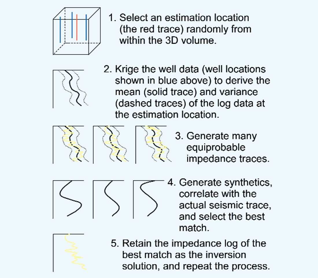
As outlined in Haas and Dubrule (1994), the log data (sonic and density) are used in the simulation of pseudo-logs at each trace within the seismic survey (figure 1). A synthetic seismogram is generated from the pseudo-impedance log and is compared with the actual seismic trace at that location. The simulation that produces the best match between the synthetic seismogram and the actual seismic trace, as defined by some quantitative measure of goodness of fit, is retained as the inversion solution at that location. The vertical resolution of the simulated log data is determined by the selection of the vertical cell size (determined by the user), not by the frequency content of the seismic data (as determined by Mother Nature). The result of the stochastic seismic inversion is a 3D volume with a seismic-like areal resolution and a log-like vertical resolution that honors both the log data and the seismic data.

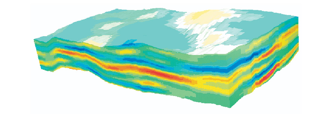
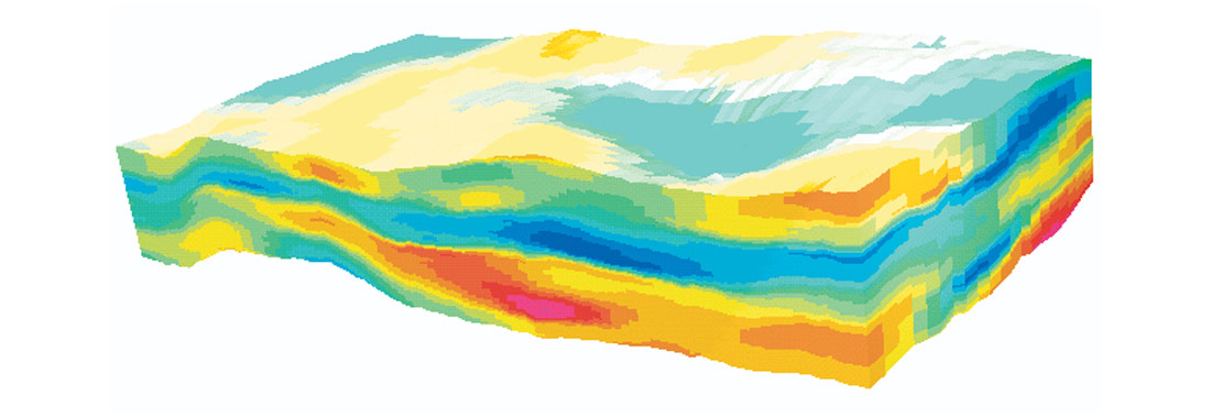
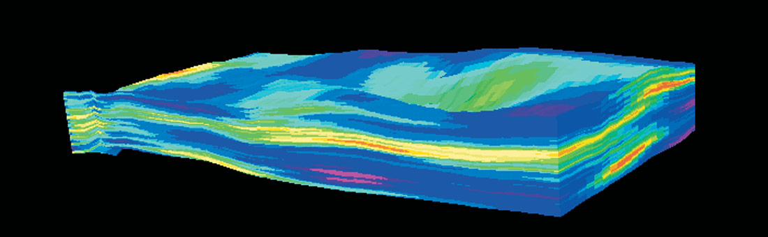
The enhanced resolution of the stochastic inversion process is evident from a visual examination of the seismic data cubes displayed in figures 2-4. Figure 2 displays the input seismic volume. Figure 3 is the result of a sparse spike estimation and recursive inversion. This inversion result displays a resolution similar to that of the input data. That is to be expected, as the vertical resolution is derived from the seismic data, and is therefore subject to the inherent limitations of seismic resolution. Figure 4 depicts the stochastic inversion cube, which displays a much finer vertical resolution than is observed in the input data or the recursive inversion result (figures 2 and 3). The overall impedance trends can be observed in both inversion results (figures 3 and 4)- layers or regions of high (red color) and low (blue color) impedance; however, the stochastic inversion result (figure 4) has a much better vertical definition within these general impedance trends.

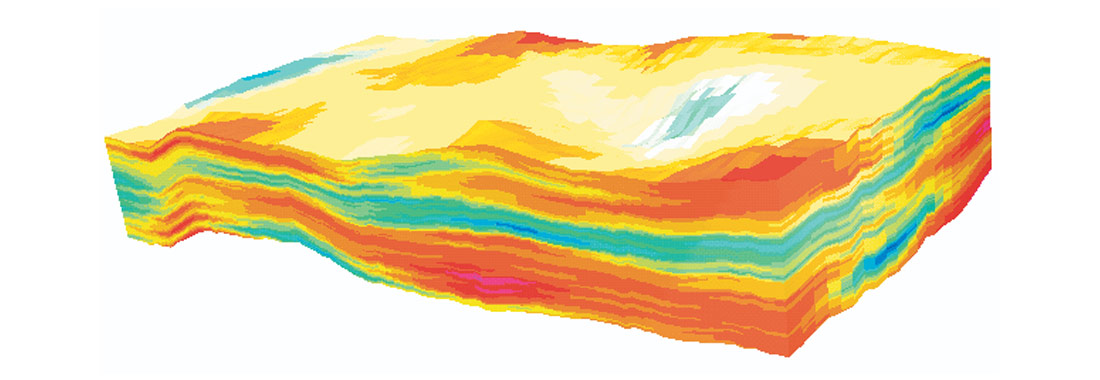
A typical stochastic inversion exhibits a vertical resolution of approximately 1-2 meters. This is generally the same order of magnitude of resolution used in constructing the petrophysical reservoir property models, and the impedance data may be used along with the well log data to generate models of reservoir properties such as porosity. Figures 5 and 6 present porosity models of the interval depicted in the previous figures. The model of figure 5 was calculated using only the log data, whereas the model of figure 6 incorporated both the impedance and porosity information. Again, although overall trends are generally similar, specific details can be significantly different. The influence of the stochastic inversion impedance model (figure 4) on the porosity model shown in figure 6 is clearly discernible, as features observed in the impedance model (figure 4) that are not present in the log-only porosity model (figure 5) are again present in the porosity model derived from both the seismic and the log data (figure 6).

In carbonate reservoirs, impedance and porosity typically exhibit an inverse relationship (Rafavich, Kendall, and Todd, 1984); in clastic reservoirs, the relationship of porosity and impedance may be complicated by additional factors, such as a lack of impedance contrast between reservoir and non-reservoir rocks or fluid effects. In the case of a clear relationship between porosity and impedance, the seismic impedance volume may be incorporated directly with well data, via geostatistics, neural networks, or other methods, to populate the cells of the petrophysical model, as was done in constructing the porosity model of figure 6. Where the relationship between impedance and porosity is murky, the impedance data may be combined with facies data to derive a facies volume. Petrophysical properties can then be distributed by facies within the overall model framework.

In summary, the impedance cube resulting from a stochastic inversion provides sufficient vertical resolution, as well as areal resolution, for use in reservoir characterization. This stochastic inversion impedance volume can be combined with log and engineering data, utilizing deterministic or statistical methods, to arrive at a reservoir model which has incorporated various data types from different disciplines (geology, geophysics, engineering) to arrive at a final, consistent 3D property model for use in reservoir characterization.