In developing an oil sands play, the task facing the geoscientist is to build a detailed characterization of a three-dimensionally complex reservoir to position horizontal wells precisely and optimally. There is usually no shortage of data to examine. In fact, terabytes of information about the reservoir are often collected. The key is to ask the data the right questions about the reservoir, and to understand the value and the limits of what the various types of information can and cannot convey.
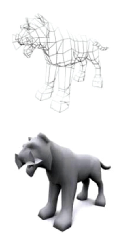
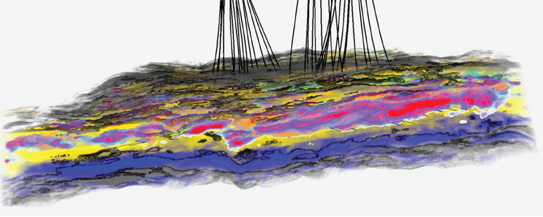
The stages of 3D animation provide an analogy for developing a meaningful depiction of the subsurface. Similar to the wireframe sketch in the first stage of a 3D animation (Figure 1), interpreted seismic horizons describe the structural framework of the reservoir. To this geometric information, elastic parameters extracted from prestack seismic data can add more detail. Attributes such as Density can help to resolve sand vs. shale, and attributes created using a multilinear regression can identify the most promising reservoir zones to be developed. With diligent modeling, these seismic attributes can be interpreted in terms of physical properties such as lithology, porosity, fluid type and fluid saturation. By extending the analysis to incorporate spectral analyses and Bayesian probabilities one can fill in even more texture and detail to the reservoir characterization.
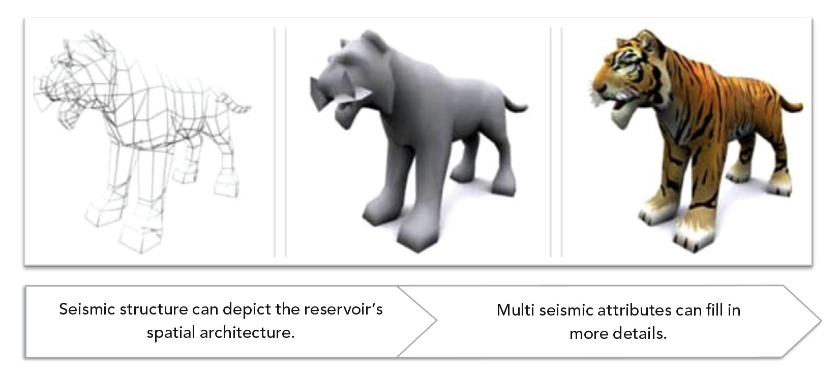
(Image source: gamedeveloper.digitalmedianet.com)
The goal is to answer key questions such as: What is the structure and architecture of the reservoir? Where is the best sand? Is it likely bitumen-charged or wet? Where are the hazards that could impair production? This article summarizes the data sources and approaches that we have found to provide the best answers so far, and sums up the must-have pieces of information. It is hoped this example illustrates some lessons learned as well as the importance for the interpreter to remain open to what the data are saying.
The prize
The Alberta Energy Resources Conservation Board estimates the oil sands initial volume in place as about 1.7 trillion barrels1. Using currently available technology and under the current economic conditions, there are approximately 170 billion barrels of recoverable oil2. But this significant hydrocarbon resource is in the form of bitumen, a semi-solid form of crude oil which is not simple to extract. An in-situ method which is being applied at a number of oil sands projects is Steam Assisted Gravity Drainage. As of November 2011, there were more than 90 active oil sands projects in Alberta using various in-situ recovery methods3.
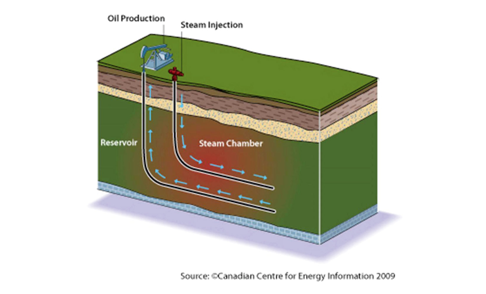
In SAGD, horizontal well pairs are drilled, and then high pressure steam is injected into the reservoir through the upper (injector) well, heating the bitumen so that it can flow down via gravity to the lower (producer) well which collects the bitumen and pumps it to the surface (Figure 2). The horizontal portions of the well pairs are generally 700 – 1000 metres in length, separated vertically by 5 meters.
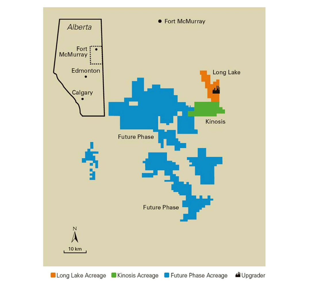
Nexen Energy ULC’s Kinosis oil sands area is 12 km south of Long Lake (Figure 3). At Kinosis, K1A development area, Nexen Energy ULC drilled 37 wells, with steam injection expected in 2014; production from these wells is expected to average 15,000 to 25,000 bpd at peak rates (Todorovic-Marinic, 2013).
About the reservoir
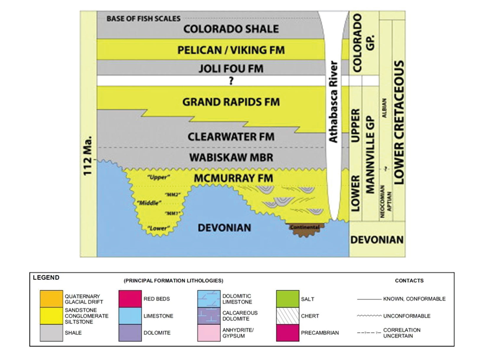
The depositional environment for the Lower Cretaceous McMurray formation at Kinosis can generally be described as one of broad valleys infilled with tidally influenced meandering river channel sands (point bar deposits) and associated sediments.
As every canoeist knows, the outer curve of a meander bend is where the river channel is deep and the current is fast, while the inner part of the meander is shallow and the current is slower. This is because sediment is eroded from an outer curve and deposited downstream as a series of point bars at the opposite shore on the inside bend of the next meander. With erosion on one side and deposition on the other, the whole channel migrates and becomes more sinuous, keeping a relatively constant width. The point bars build by lateral accretion via the simultaneous processes of lateral and downstream meander growth. Deposits at the base of the point bar sequence are generally sandstone-dominated and fine upwards.
When the river floods and overflows its banks, very fine sediments from the floodplain can be deposited. Over time, these stacked point bar sandstones are interbedded with dipping mudstones – characterized by highly variable dip – known as inclined heterolithic stratification, or IHS (Fustic et al, 2012).
Some of these mudstones extend laterally for hundreds of meters, and can be permeability barriers between the injector and producer wells making a portion of the producer well’s length ineffective. Sometimes the mudstones do not have a long lateral extent – one could say they are ‘patchy’ rather than a ‘blanket’ shale. In the early 2000’s it was thought that such discontinuous thin mudstones would act like baffles rather than barriers to steam chamber growth (the steam would deflect around them). But production data from Long Lake Long has shown that patchy discontinuous shales – if there are enough of them – can, in fact, act as barriers to SAGD (Arnold, 2011). Therefore placing both injector and producer wells in continuous, high permeability crossbedded sand lithofacies is best, if possible.
Further, one observes rapid lateral changes in bitumen saturation, even between closely spaced wells. And one may observe variable structure of oil-water contact (to be discussed in separate paper). The point to be made is that the reservoir presents complex, rapid local variations.
It is therefore important to use suitable tools to map sands, identify barriers and develop as detailed a 3D model as possible of the reservoir. Underestimating the three dimensional complexity of the reservoir properties could be a very expensive mistake.
Filling in details
One begins by describing the reservoir in terms of its geometric structure. Interpreted horizons from a conventional 3D seismic stack volume provide the wireframe of the McMurray formation (reservoir), as well as the structure of underlying and overlaying formations, which may have influenced the depositional environment.
The next steps are to add more seismically-derived details to the reservoir picture. An amplitude horizon map guides you to the areas to focus on for more detailed work such as spectral analyses.
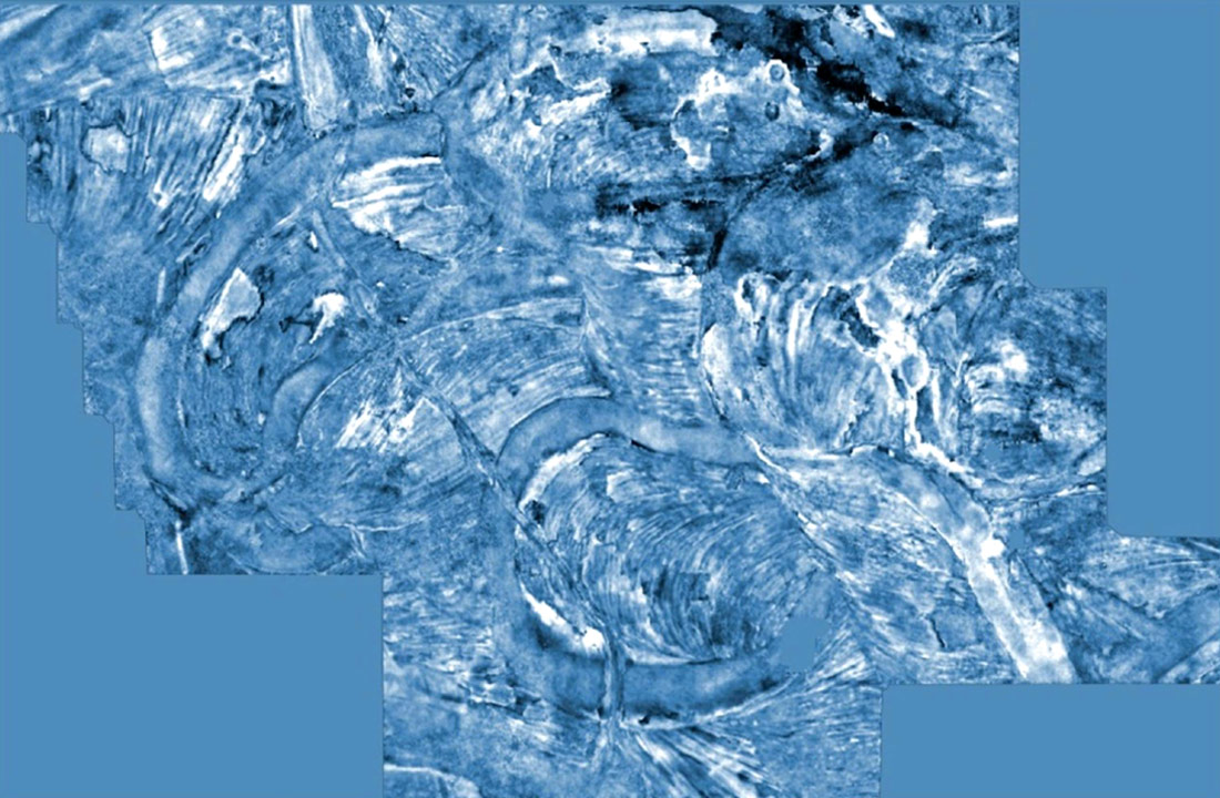
Spectral Decomposition is a technique to deconstruct the seismic data into discrete sub-band frequencies. Full bandwidth seismic is skewed towards what the dominant frequency of the seismic wavelet can ‘see’, but decomposition into discrete bands may allow spatial details in geologic heterogeneity to be ‘illuminated’ at various frequencies of the seismic data. In this way, Spectral Decomposition can expose stratigraphic and structural edges, layering complexity and relative thickening and thinning.
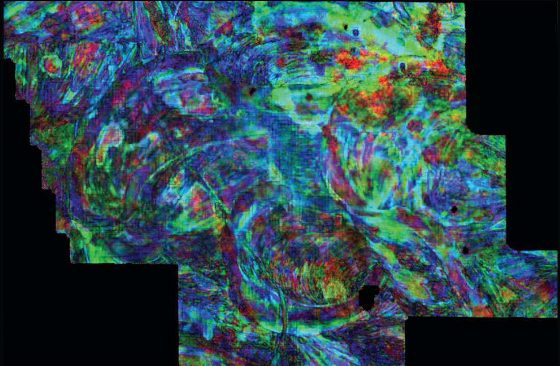
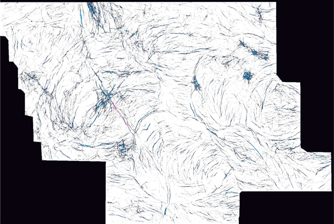
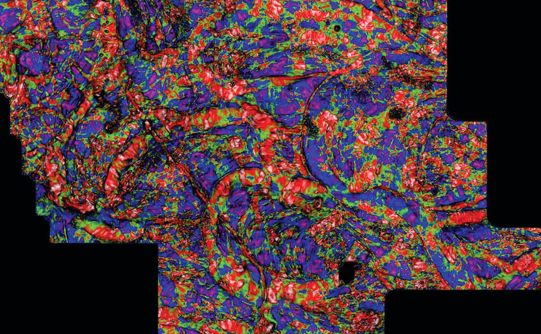
Dip Azimuth volumes – extremely localized estimates of dip magnitude and dip direction at the McMurray surface – were computed from the 3D seismic data to estimate the dips of strata within a point bar sequence. One may combine Dip Azimuth and Spectral Discontinuity volumes. The resulting image reveals, in considerable detail, the internal structure of the point bar deposits. Because interbedded shales (mudstones) between the injector and producer wells can act as barriers impeding SAGD, it is important to identify this expensive hazard for optimal well placement.
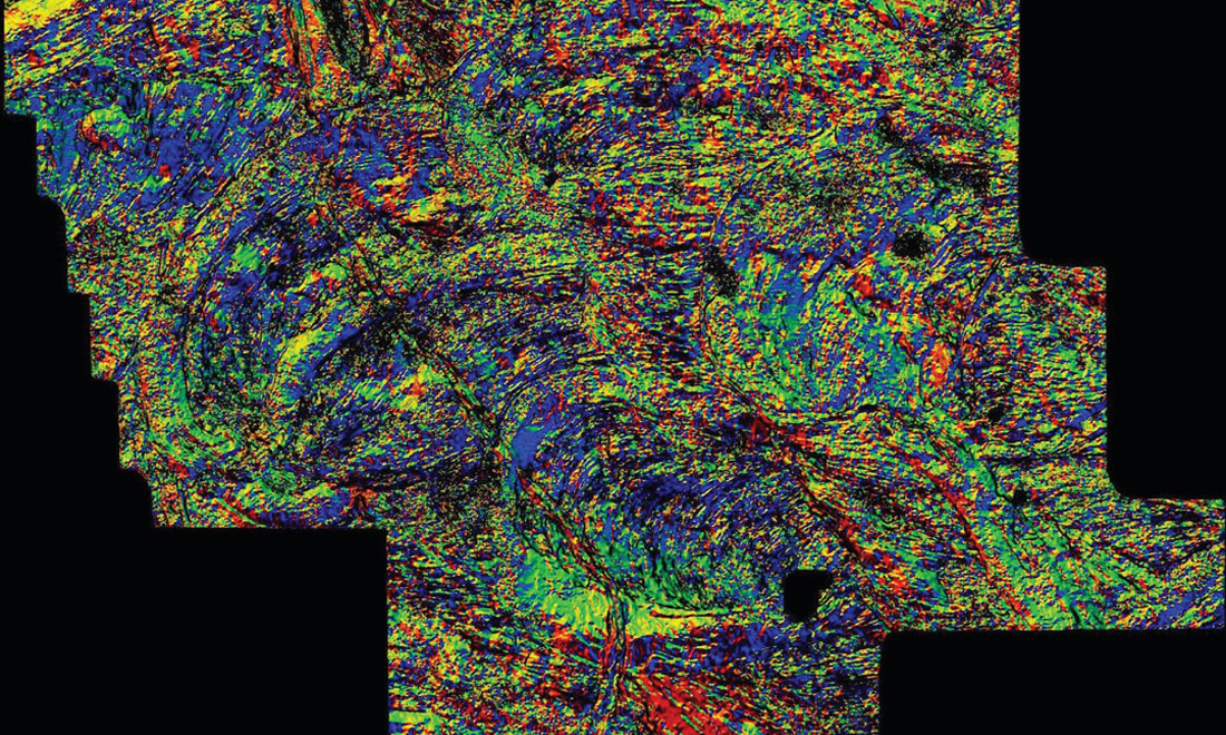
Ant-Tracker, an algorithm to perform automated fault interpretation, can be used to delineate local discontinuities (Pedersen et al.,2002).
Curvature, a measurement of the degree of bending of a reflecting surface, indicates localized structure, ranging from dome-shaped hills to bowl-shaped valleys. Curvature may suggest the morphology of the local structure: mud vs. sand, in this case. Assuming differential compaction, the domes – localized structural highs – correspond to areas of a channel which are sand-filled, while concave bowls correspond to softer mud-fill. This interpretation, based on a purely geometric attribute, can be compared to the results from spectral and inversion tools.
Adding in details from multi-attribute analysis

To add information of subtle features we begin by incorporating multi-attribute analysis, which uses statistical analysis to learn seismic attribute / well log relationship at well locations. It then applies that learned relationship throughout the 3D volume to produce a 3D volume of the predicted log property (Hampson et al., 2001). It would be difficult to assess from the seismic stack alone the quality of the reservoir – sand vs. shale, bitumen-saturated sand vs. wet sand – but all of this becomes clearly defined in the 3D volumes of log properties.
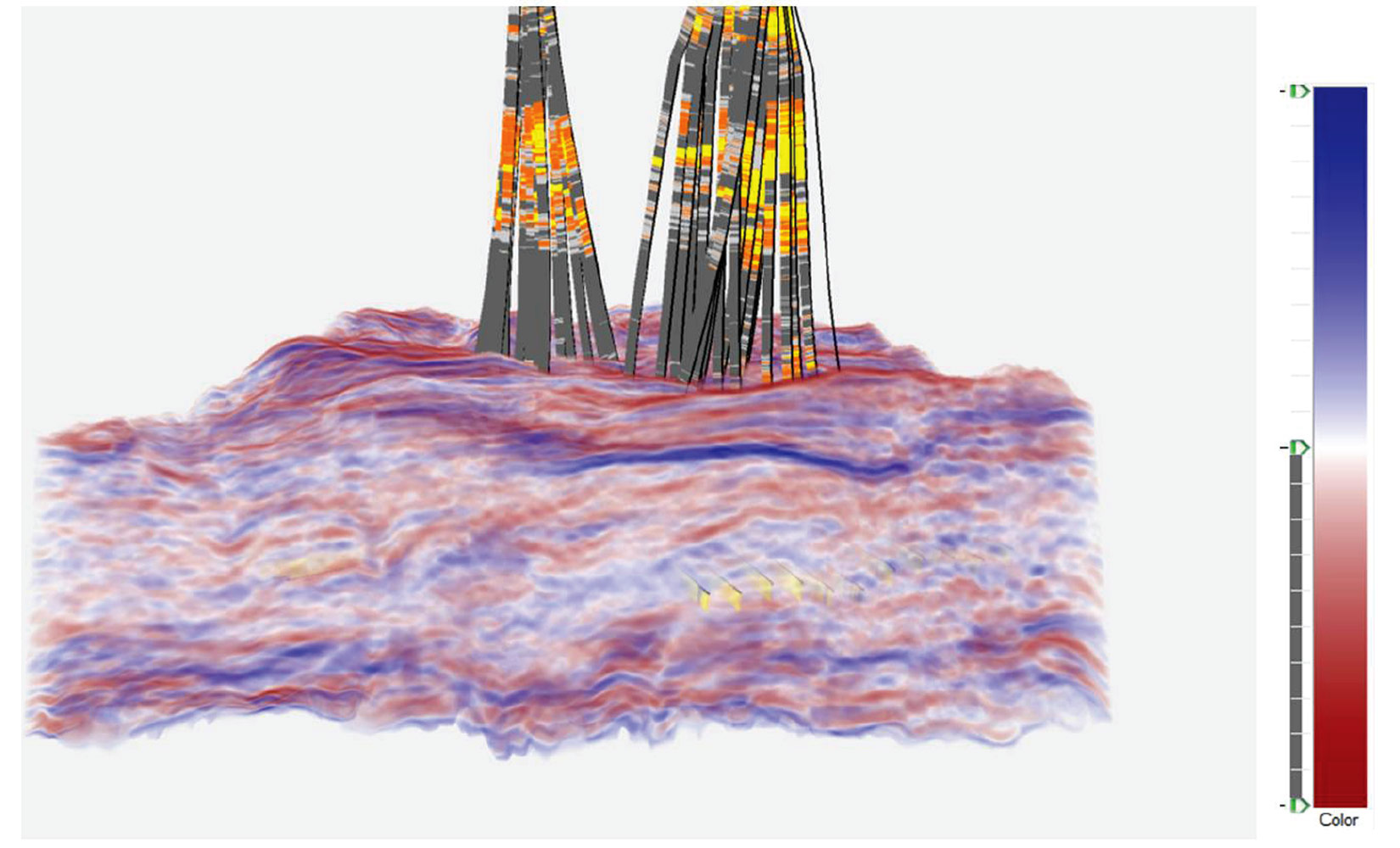
In oil sands reservoirs, it has been observed that bulk density is strongly related to properties such as lithology (sand vs. shale discrimination) and porosity (Gray, 2011). Density and/or Vshale 3D volumes can be used to provide detailed intra-well information to delineate the clean sand in this reservoir (Figure 10).
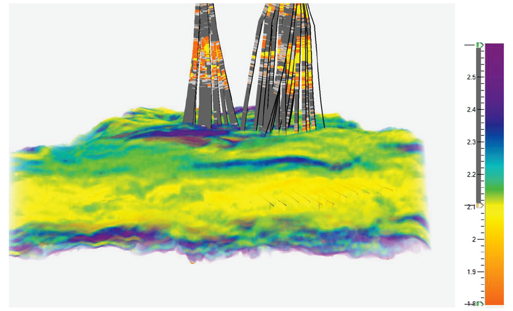
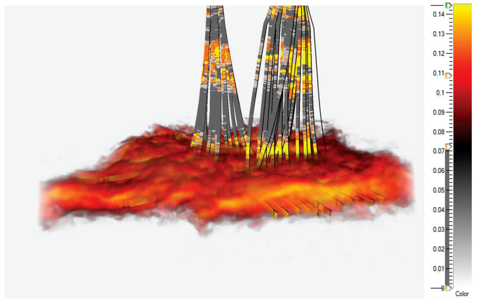
Next, we seek to answer the question: is the sand bitumen-charged or wet? The best 3D log property to answer that question is WTAR, log derived weight-percent bitumen which is the ratio of the mass of oil to the total formation mass. What is considered to be good reservoir has WTAR between 6-12%. A 3D volume of this log property can be generated using multi-attribute analysis (Figure 11).
Keep it simple
It is helpful to remember that, despite the complexity of the reservoir and data, there are essentially two simple questions that one wants to answer: Where is it good (or probably good)? And where is it hazardous?
To this end, petrophysical analysis is performed at each well location to develop rule-based facies classifications. These can then be incorporated into a lithology prediction workflow to determine where, and with what probability, these facies classifications are found in the seismic volume (Russell, 2004). The approach is described below.
Where is it good?
To answer this question, one must first quantify what ‘good’ means. In the McMurray reservoir, the quality of a reservoir zone can be defined in terms of its Vsh, Sw, and thickness. An Energy Resources Conservation Board report released in 2011 summarizes it this way: “The quality of an oil sands deposit depends primarily on the degree of saturation of bitumen within the reservoir and the thickness of the saturated interval. The level of bitumen saturation within a reservoir can vary considerably, decreasing as the shale or clay content within the reservoir increases or porosity decreases. A greater volume of water within the pore space of the rock also decreases bitumen saturation.”
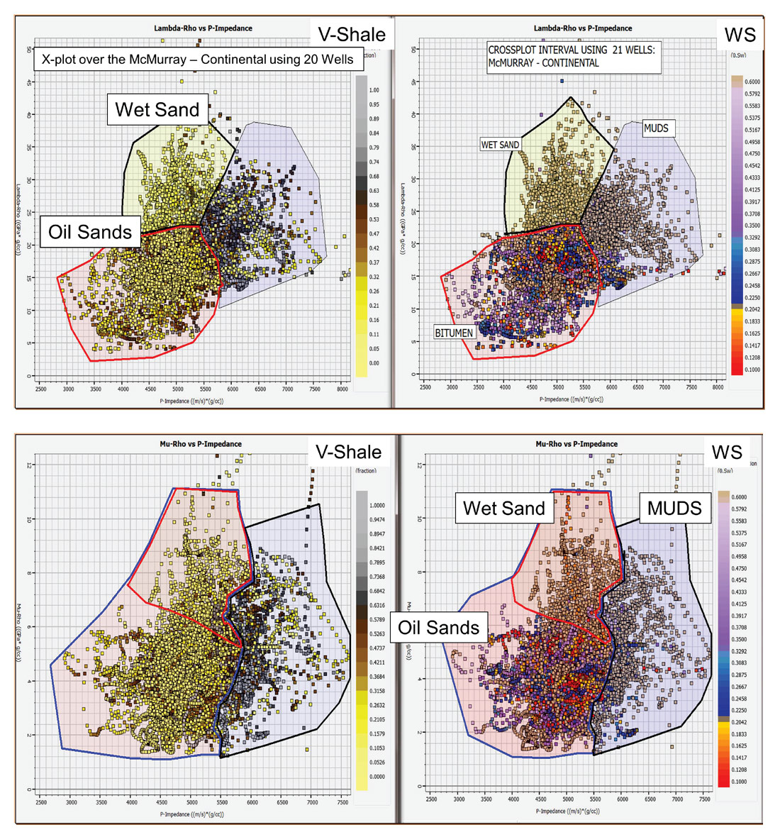
In the case of Kinosis, for each well in the field careful analysis using well logs, FMI data, and core sample descriptions has been carried out to establish petrophysical rule-based cutoffs to define the reservoir sand facies (Figure 12).
In the inter-well space, where is it probably good (and what’s the probability)?
Following proper QCs at the well locations, the above petrophysical rule-based classifications are incorporated in a Bayesian approach and applied to seismic inversion volumes to generate a probability volume for each facies classification (Nieto et al, 2013). A composite Most Probable Petrofacies volume is also generated (Figure 13).
Drilling results
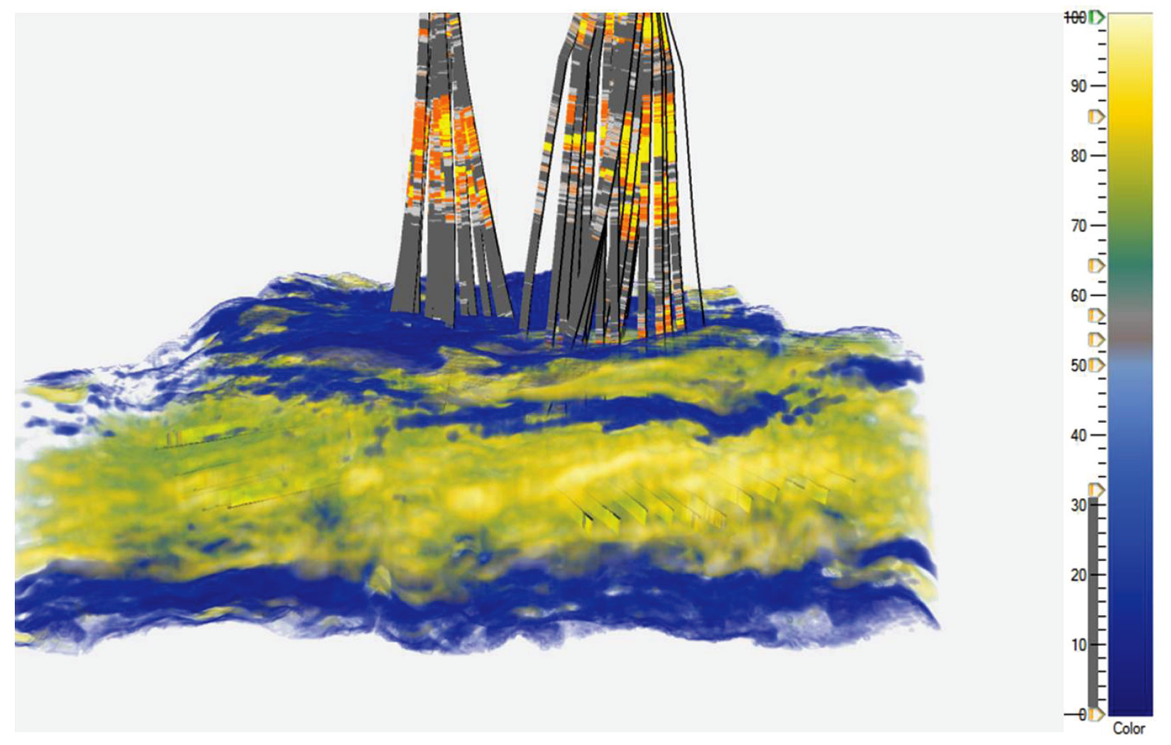
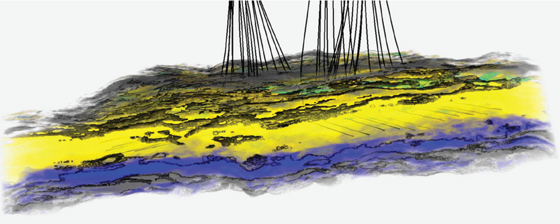
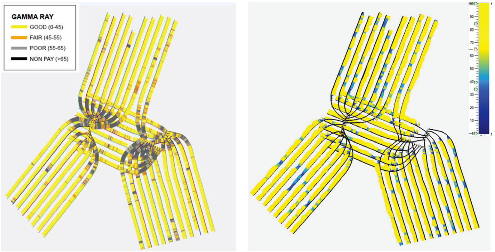
The fleshed-out description of the reservoir that was derived from the above workflow was used to guide the positioning of SAGD horizontal well pairs in the complex Lower Cretaceous McMurray reservoir. Figure 16 shows the actual gamma ray logs along the well paths (left), and the predicted ‘good reservoir’ as extracted from the Oil saturation probability volume along these same paths.
Conclusions
Things can get really complicated really quickly when the goal is to build a detailed characterization of a three-dimensionally complex reservoir to position horizontal wells. Keep in the forefront the questions you want the data to answer: What is the internal structure of the reservoir? Where is the best sand? Is it likely bitumen-charged or wet? Where are the hazards? Extract as much information as possible from the seismic, remembering that no single seismic attribute is sensitive enough to distinguish safely between sands, shale and fluid saturation. Integrate a set of input attributes in a neural network approach to determine the optimal combination to reliably discriminate things like sand vs. shale, and So v.s Sw, and qualify the seismic estimates with direct measurements from wells.
1 Canadian Centre for Energy Information, http://www.centreforenergy.com/AboutEnergy/ONG/OilsandsHeavyOil/Overview.asp?page=4
2 Government of Alberta Department of Energy, http://www.energy.alberta.ca/OilSands/1715.asp; and
3 Government of Alberta Department of Energy, http://www.energy.alberta.ca/OilSands/791.asp

Acknowledgements
The authors would like to thank Bogdan Batlai, Elizabeth Earl, James Alison, Paul Garossino, Kevin Pyke, Wendy Akins and Farid Kassam as well as the whole Kinosis Development team for their assistance in this work.
We would also like to thank Nexen Energy ULC for their kind permission to show these data, and Hampson-Russell and OpenGeoSolutions for the work they have done on these projects.


Join the Conversation
Interested in starting, or contributing to a conversation about an article or issue of the RECORDER? Join our CSEG LinkedIn Group.
Share This Article