Abstract
Microseismic or passive seismic monitoring during hydraulic fracturing processes involves recording 3C seismograms produced by microearthquakes associated with breaking rock. By analyzing the data to locate hypocenters where the breakage occurs, geophysicists enable reservoir engineers to follow the growth and evolution of the fractured rock volume in time and space. Because of low signal-to-noise ratios in recorded microseismograms and other factors, the estimated hypocenter locations are often inconsistent and inaccurate. Different algorithms and processing flows applied to identical field data often produce radically different estimates of source locations. In a real world scenario, it is difficult or impossible to ascertain which of several different but ostensibly viable solutions is true, since there is no independent validation. However, synthetic data can be generated with known source locations and recording configurations in different velocity structures. Such synthetic data can be used for objective testing of the reliability of various location algorithms and processing flows.
Introduction
Passive monitoring of microseismic events produced by rock bursts or induced by hydraulic fracturing has been used for many years. The technique has proven valuable in the development of shale-gas reservoirs because analyzing microseismic data to locate fracture points allows reservoir engineers to follow the progress of a hydraulic-fracture stimulation project. However, locating fracture-point hypocenters using microseismic monitoring and analysis is often plagued by uncertainties and inaccuracies. Different algorithms such as migration (Chambers et al., 2008), inversion (Wong, 2009; Gharti et al., 2010; Wong et al., 2010), and back-projection (Han et al., 2010) applied to the same dataset can produce radically different estimates of source locations. This is especially true if the acquisition aperture of the recording array is small in angular extent, and if the microseismic arrivals are weak compared to the noise.
We have designed and created synthetic microseismic datasets with varying random noise levels for testing the reliability of different source location algorithms when used with noisy data. Three–component microseismograms with sources and receivers embedded in horizontally layered velocity structures can be generated either by ray-tracing (RT) and convolution, or by 2D finite-difference (FD) modeling. The RT-modeled seismograms include direct and head-wave arrivals, but no reflected arrivals. The ray-tracing method can approximate some effects of TTI anisotropy in the layers. Traces from FD modeling include reflected as well as direct and head wave arrivals, but at present the FD code we use does not address effects due to anisotropy.
In the modeling, various receiver configurations can be used to record events from subsurface sources embedded in horizontally- layered P and S velocity structures. Such structures adequately represent the geological setting for many realworld hydraulic fracturing projects. Gaussian noise and harmonic noise are added to the synthetic traces to simulate microseismograms with different signal-to-noise levels. The modeled data are stored in files with SEG-2 format to conform to field-recorded data files.
Hypocenter location techniques require accurate relative amplitudes of the x, y, and z components of P-wave arrivals in order that the direction cosines of the propagation vector at receivers may be estimated. They also require accurate arrival times of the P and/or S arrival times relative to some reference time that is not the actual time of occurrence t0 of the associated microseismic event. Our modeling schemes do not yield true absolute amplitudes for the receivers, but the relative amplitudes of the direct P-wave arrivals for a given 3C geophone are accurate, as are the arrival time moveouts of all modes. Since the hypocenter coordinates for the synthetic data are known, we can use the synthetic data to evaluate objectively the effectiveness and accuracy of different location methods for different recording geometries and under various signal-to-noise levels.
Velocity-Density Model
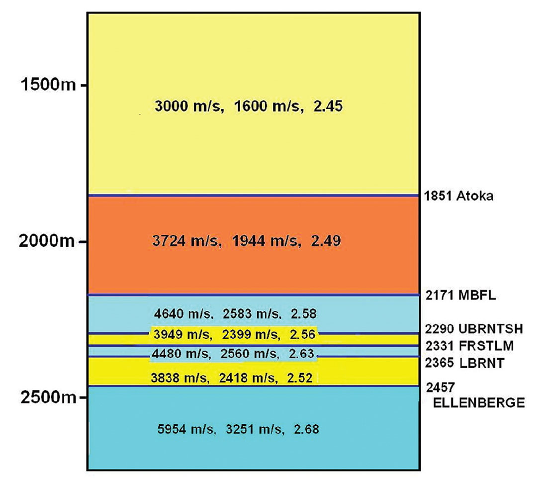
Figure 1 is a diagram depicting a horizontally-layered model used for ray-trace modeling, showing P-wave velocity, Swave velocity, and relative density for each layer. The model is a representation of geological structure typically encountered by hydraulic fracturing projects in the Barnett shale in Texas. The tops of the shale layers are located at depths of 1851 m, 2290 m, and 2365 m. The lower Barnett shale at 2365 m is a gas shale that is a target of hydraulic fracturing stimulation. The seismic parameters of the model are listed on Table 1.
| Layer Number | Top of Layer (m) | P velocity (m/s) | S velocity (m/s) | r (gm/cc) |
|---|---|---|---|---|
| Table 1. Velocity-density model for calculating microseismic data files using ray tracing. A visual representation of the model is shown on Figure 1. | ||||
| 1 | 1500 | 3000 | 1600 | 2.30 |
| 2 | 1851 | 3724 | 1944 | 2.45 |
| 3 | 2171 | 4640 | 2583 | 2.49 |
| 4 | 2290 | 3949 | 2399 | 2.58 |
| 5 | 2331 | 4480 | 2560 | 2.63 |
| 6 | 2365 | 3838 | 2418 | 2.52 |
| 7 | 2457 | 5854 | 3251 | 2.68 |
| 8 | 3000 | 5854 | 3251 | 2.68 |
Source-Receiver Geometry
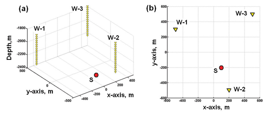
A possible recording geometry for 3D microseismic monitoring is shown on Figure 2. Arrays of three-component geophones can be placed in one or more observation wells. The wells may have vertical, slanted, and even horizontal sections. The number of geophones in the arrays and the spacing between the geophones in the arrays can be varied. Microseismic sources can be placed at any depth and distance from the observation wells. Examples will be shown for a single vertical array with 16 or 24 geophones spaced at intervals of 25 m.
Seismograms Produced by Ray-Tracing
Ray-tracing through the layered velocity model gives P and S raypaths between the source and receivers as well as the travel times and incident directions at the receivers. An example of raytracing through a homogeneous isotropic P-wave velocity field is displayed on Figure 3, where all the layers have an identical velocity of 4000 m/s. The microseismic source coordinates are (xs, ys, zs) = (100 m, -200 m, 2425 m). The receiver coordinates are (xr, yr, zr) = (500 m, 500 m, 2000 to 2575 m), with spacing Δz = 25 m. They are associated with well W-3 on Figure 2.
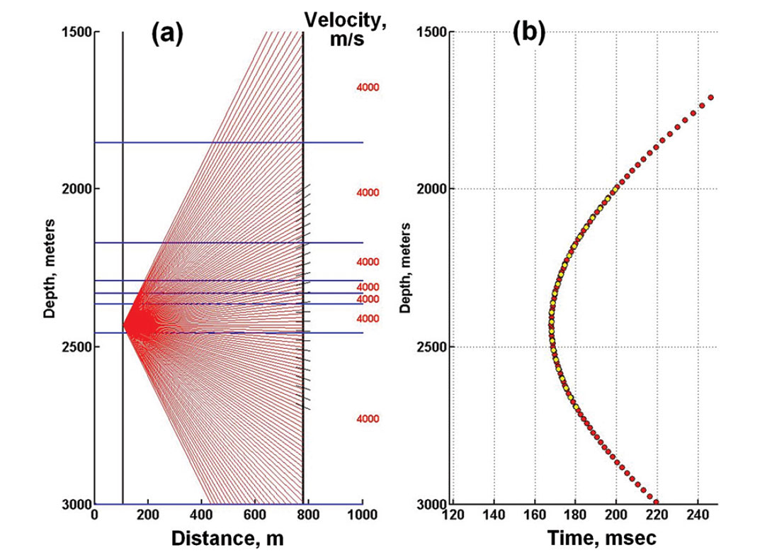
Figure 3a shows the network of rays traced from a source in the stimulation well on the left to receivers in the observation well on the right. The horizontal scale is distance across the 2D plane spanned by the two wells. Figure 3b shows that the arrival times for these rays fall on a perfect hyperbola, as expected for a uniform velocity medium.
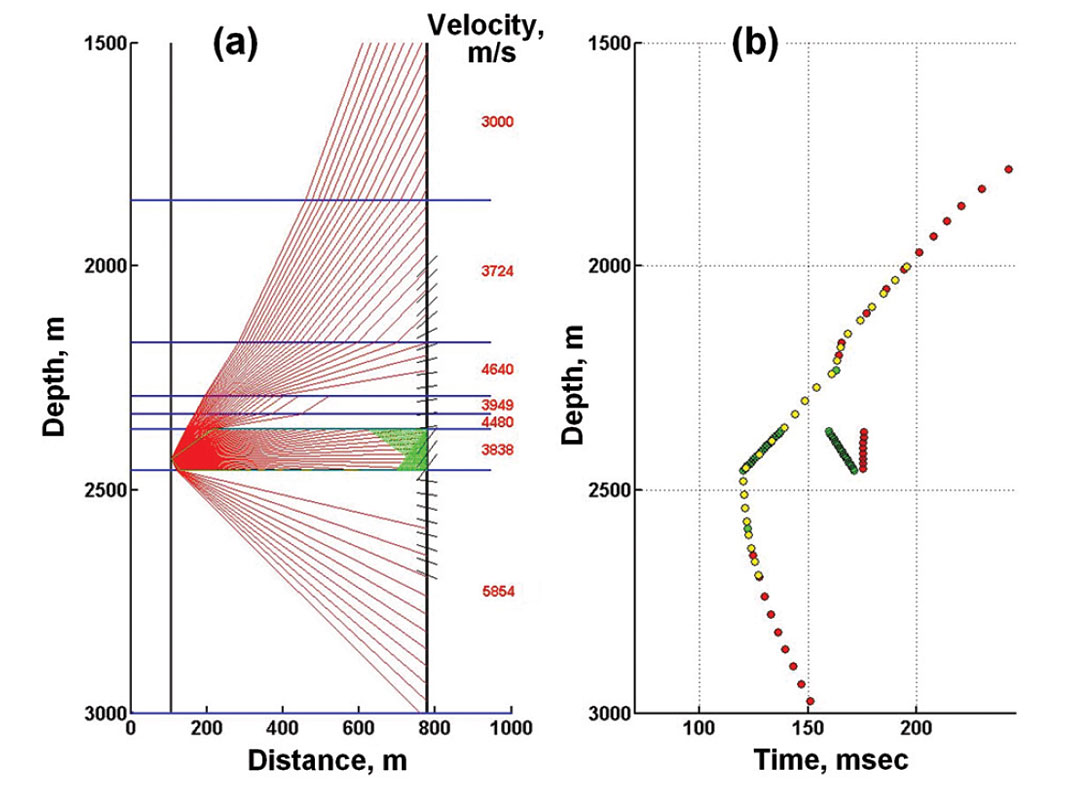
On Figure 4, we see the raypaths and arrival times when different velocities are assigned to the layers. Raypath refraction according to Snell’s Law occurs at the layer boundaries, and the arrival times no longer fall on a hyperbolic curve. Raypaths to particular receiver locations can be found by interpolation of rays produced by shooting from the source at many angles (interpolated positions are indicated by the short black lines). They may also be found more directly by a ray-bending method that follow Fermat’s principle of minimum time. We have also plotted (in green) head wave raypaths and arrival times. The propagation directions of the first P-wave arrivals at the receivers are represented by the short slanted lines on the observation well. A similar figure showing a network of traced S wave arrivals can also be drawn by assigning the S velocity values on Table 1 to the layers.
To produce microseismograms, wavelets approximately scaled for geometric spreading are placed at the appropriate arrival times. Both the P and S wavelets have the form

This is the response of a damped harmonic oscillator. Specific values for the parameters f and κ are arbitrary; we have chosen f = 300 Hz, κ = 80/s for the P arrivals, and f = 200 Hz, κ = 50/s for the S arrivals.
For each receiver, three-component (3C) traces are synthesized with scaled amplitudes for the P and S direct arrivals. The noisefree x-y-z P-wave amplitudes for each receiver are scaled so that direction cosines derived from them using hodogram analysis will always point back to the source. The 3C amplitudes for the S wave arrivals are forced to be in the correct proportions so that their motions are transverse to the propagation directions at the receivers. Note that the 3C amplitudes of the nnnnnnS wave arrivals cannot be used to determine the propagation direction unambiguously. The relative amplitudes on the modeled seismograms between different modes (P and S direct arrivals, and head waves) are arbitrary and have no significance. Our ray-trace modeling technique produces microseismograms that show only direct arrivals and head-wave arrivals; for simplicity, we have chosen not to include reflected or guided wave arrivals.
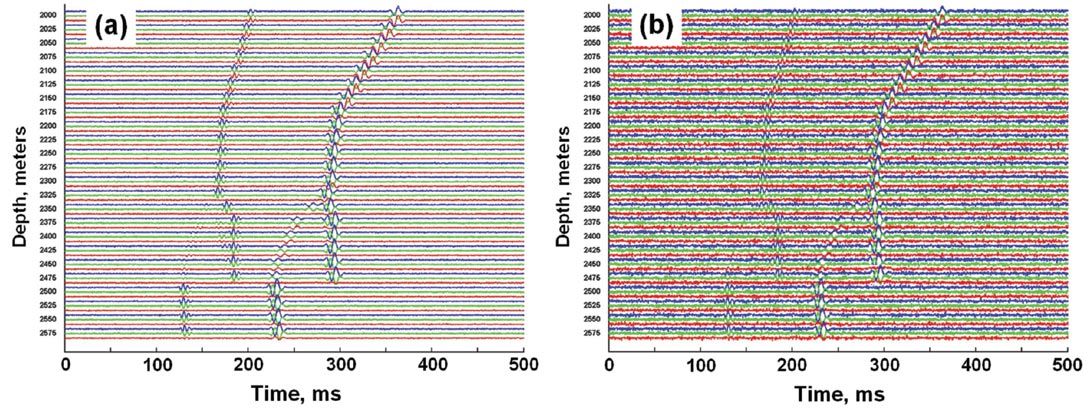
Figure 5 shows gathers of 3C seismograms for the source location and geophone positions for well W-3 on Figure 2. The seismograms have been plotted as color-coded triplets for each receiver, with blue-green-red denoting the x-y-z components, respectively. The amplitudes of the P arrivals have been set to 0.5 times the amplitudes of the S arrivals. The head wave amplitudes have been arbitrarily set to 0.25 times the direct arrival amplitudes. The SNR values are set relative to the direct P wave amplitudes. The low-noise traces have SNR = 10 (Figure 5a), while the noisy traces have SNR = 3 (Figure 5b). The higher noise levels on Figure 5b completely obscure the weak head wave P arrivals.
Ray Tracing Through Anisotropic Layers
Byun et al. (1989) and Kumar et al. (2004) have developed formulae for group velocities of quasi-P (qP) waves that can be used to trace qP rays through anisotropic horizontal velocity layers with tilted transverse isotropy (TTI). The Byun approximation for quasi-P wave group velocities in VTI media is given by:
where Vv, Vh, and V45 are the group velocities in the vertical (∅=0°), horizontal (∅=90°), and 45° dip angle directions. For the isotropic case, a1 and a2 are identically zero. Kumar et al. (2004) and Casasanta et al. (2008) compared qP group velocities, raypaths, and travel times using Equations 1 to 4 with results from the exact treatment of VTI and from the Thomsen approximations (Thomsen, 1986). They showed that the Byun formulation gave results closer to those derived from the exact treatment of VTI. Tilted transverse isotropy (TTI) can be simulated by tilting the VTI symmetry axis by an angle ψ in the x-z plane (Kumar et al. 2004). Equation 1 still applies, but the angle ∅ is replaced by (∅+ψ),

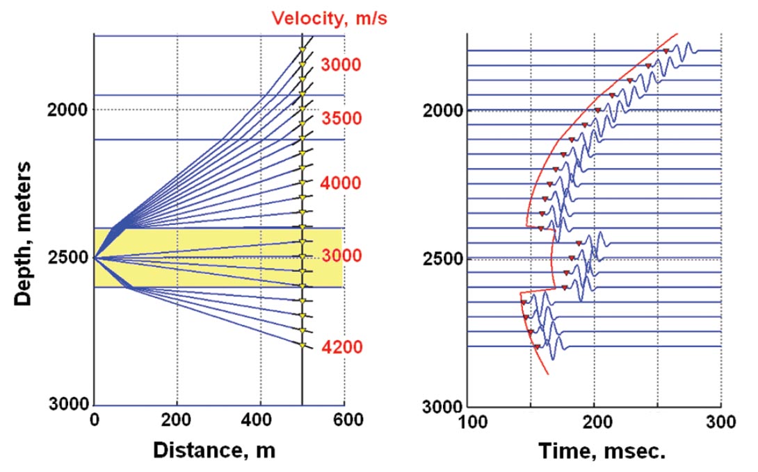
Figure 6 shows an example of synthetic P arrivals obtained when the low velocity layer shown in yellow has its VTI symmetry axis tilted clockwise by 30º. Figure 6a shows the raypaths traced from a source on left to an array of receivers on the right. On Figure 6b, the red curve represents the arrival times if all layers have isotropic velocity values as shown. The small red triangles are the arrival times when the layer just below 2400 m (shown in yellow) is TTI. Even though there is only a single TTI layer, there is significant deviation of the TTI arrival times from the isotropic times. Clearly, the effects of anisotropy must be taken into account if one were to use the arrival times to locate a microseismic hypocenter. If a receiver happens to be located in an anisotropic layer, the direction cosines derived for the P-wave 3C amplitudes will not define a vector parallel to the propagation vector.
Anisotropy for shear waves can be included in ray-tracing schemes by using formulae similar to Equations 1 to 5 for the quasi-shear group velocities qVsv and qVsh. Approximations for the quasi-shear phase velocities were given by Thomsen (1986).
Seismograms Produced by 2D Finite Difference Code
Seismograms can also be produced by a 2D time-stepping finite difference (FD) code for isotropic media (Manning, 2008; 2007). Finite difference elastic modeling will automatically generate direct P and S arrivals as well as all the refracted, reflected, and converted arrivals due to the boundaries in the velocity-density model. Because of stability issues related to FD modeling and the desire to have reasonable execution speed and grid array size, we have restricted the dominant frequencies in the synthetic seismograms to be 300 Hz or less. These are low compared to frequencies exceeding 500 Hz commonly observed for microseismic events associated with events caused by hydraulic fracturing.
Since we use a 2D code, the relative amplitudes and phases of the various arrivals will not be correct for microseismic sources in 3D space, but the kinematics (i.e., arrival times) will be correct, and low-amplitude seismograms in seismic shadow zones will be modeled. For the direct P arrival, the x and z amplitudes will be correct in the 2D plane. To simulate the x and y amplitudes in 3D space, the P-wave x amplitudes from the 2D code are split by applying the direction cosines from the source to each receiver. This is a straightforward calculation, since for horizontally-layered velocity media, the projection of the propagation vector between the source and receiver onto the x-y plane is a straight line.
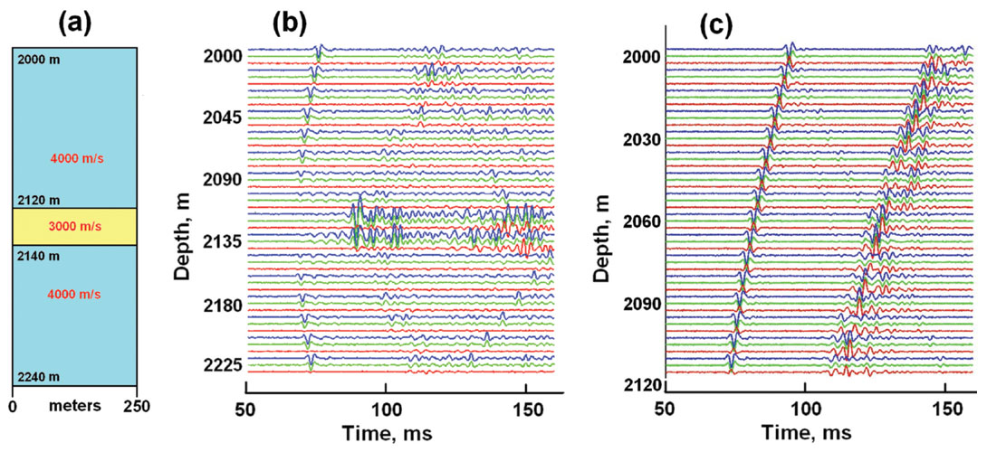
Figure 7a shows a simple three-layer model for the finite difference calculations. Figures 7b and 7c displays two gathers of microseismic traces for a source in the 3000 m/s shale layer at a depth of 2135 m shooting into vertical arrays located 250 m horizontally from the source. The P-wave velocities of the layers are shown on the figure; the S-wave velocities are 2500 m/s, 1875 m/s, and 2500 m/s; the relative densities are 2.7, 2.5, and 2.7. The resulting finite-difference seismograms on Figure 7b are rather complex, with guided waves, mode conversions, and grid boundary artifacts clearly visible. Figure 7c displays seismograms for an array that lies entirely above the low-velocity zone representing a shale zone subjected to hydraulic fracturing stimulation. Such a recording configuration is often used so as not to penetrate the gas-producing stratum with an observation well. For clarity, the x-y-z component microseismograms on Figure 7c have been plotted separately (with a modest amount of random noise) on Figure 8.

Noisy Microseismograms
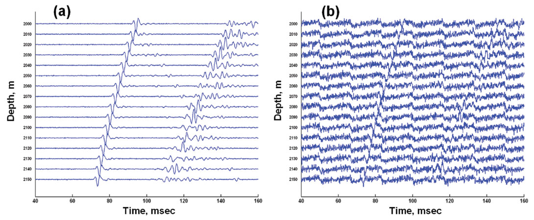
Microseismic arrivals on real field-recorded traces are weak, and are often at least partially obscured by random noise, power line harmonics, and vibrations from machinery such as downhole pumps. To simulate these effects at different signal-to-noise ratios (SNRs), we add various levels of Gaussian noise and 60 Hz harmonic interference to our synthetic traces. Figures 9a and 9b show how strong noise affects the quality of microseismic gathers. It would be a challenge to locate a hypocenter reliably using an automatic process to analyze the data on Figure 9b.
For a given microseismic source, the ray-traced arrival times give the correct absolute arrival times at the receivers. However, in recording real microseismograms, the arrival times recorded by a receiver array for each microseismic event are randomly delayed by an unknown time t0. Accordingly, in order to provide a realistic simulation, we also apply a random delay for the data corresponding to a microseismic event.
File Structure
The 3C seismograms are stored in files with SEG-2 format (Pullan, 1990). The first three traces are the x, y, and z components for the first geophone, the next three traces are the x, y, and z components for the second geophone, and so on. The coordinates of the 3C geophones are recorded on the corresponding trace headers along with a time stamp. The source coordinates may or may not be written into the file headers, depending whether or not a blind test is desired.
Every synthetic microseismic file contains P and S arrivals for a single microseismic event. Each file contains 96 seismograms if the receiver array consists of 24 three-component geophones, or 48 seismograms if the array contains 16 geophones. Receivers can be placed anywhere on the surface of the layered earth, either randomly or in regular arrays. They may also be placed in deep or shallow wells with vertical, slanted, or horizontal sections. Datasets can be produced for receiver arrays in one, two, or three observation wells. Receiver spacings can be set to 10m, 25m, or 50m. Gaussian noise and multi-harmonic noise (simulating interference from pumps or power lines) may be added for testing how well location algorithms perform with microseismograms with various signal-to-noise ratios. Typically, sampling time is set to 0.25 ms, and each seismogram is 12,000 points or 3000 ms long. All arrivals on a particular file are delayed by a time t0 randomly set to a value between 100 ms and 2975 ms, reflecting the fact that the actual event time is unknown.
Location Example: Back-Projection Technique
With a suite of synthetic microseismic data, we can apply particular location algorithms and processing flows in order to estimate the coordinates of the hypocenters. The SEG-2 files are read to extract the 3C microseismograms along with the receiver array geometry. Either manual or automatic time picking is applied to identify the direct P and S arrivals and obtain the relative arrival times. The x-y-z P-wave arrival amplitudes are processed to obtain the direction cosines of the propagation vector at each receiver. These relative arrival times and direction cosines are the observable quantities that allow us to locate the hypocenters of the microearthquakes, assuming that the velocity structure is well known.
Many different location schemes can be used to estimate the coordinates of a hypocenter. A common procedure that works well in a medium with homogeneous P and S velocities is to use the propagation vector direction cosines at a receiver to point towards the source, and the differences between the P and S arrival times to determine a distance to that source. With an array of receivers, a unique set of source coordinates can be found in a least-squares sense.
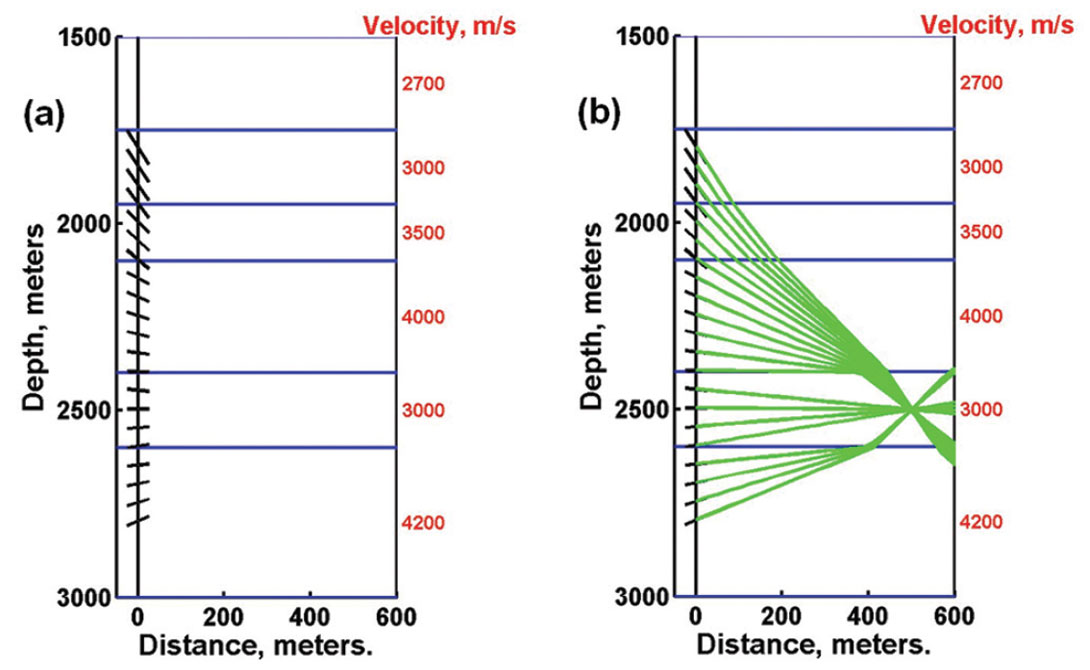
When the velocity medium is inhomogeneous, more elaborate analyses must be applied for hypocenter location. As an example, we will present a back-projection method that uses only the propagation directions derived from P-wave 3C amplitudes at receivers and not the arrival times (Han, 2010; Han et al., 2010). Figure 10a displays a 2D view of an array of receivers located in a vertical well with the propagation directions indicated by short black lines. Figure 10b shows the vector directions back-projected by ray-tracing through the (known) layered velocity structure. Since the original 3C data have high SNRs, the derived direction cosines are accurate and back-project to a common intersection point that coincides with the source hypocenter.
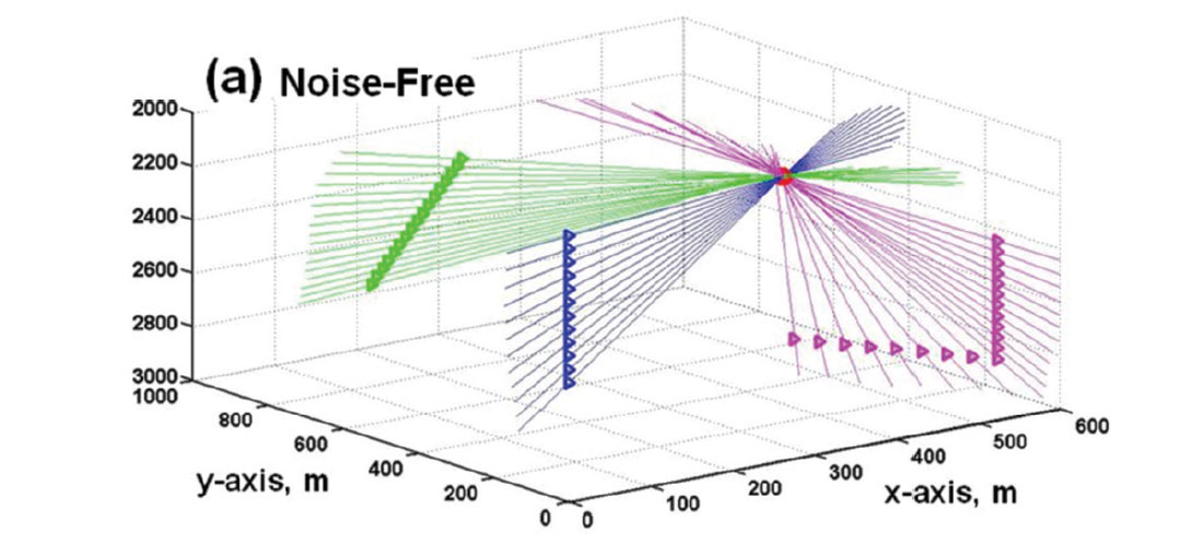
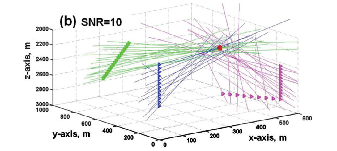
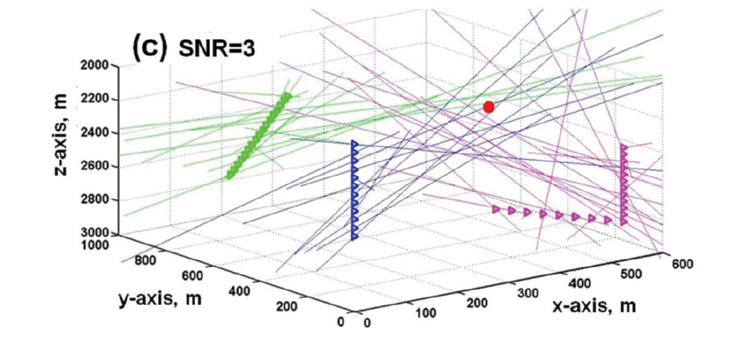
Figure 11 is a 3D view of 44 receivers in a homogeneous velocity structure. The receivers are situated in a vertical well, a slanted well, and a well with a horizontal leg. From each receiver is a straight raypath back-projecting along propagation directions estimated from the three component P-arrival amplitudes. When P-arrival amplitudes have high SNRs, the back-projected straight lines in 3D all intersect at the hypocenter location (Figure 11a). When there is moderate random noise in the microseismograms, the back-projected vectors do not intersect at a common point, but they converge towards a volume surrounding the microseismic source (Figure 11b). When the random noise is more extreme, there appears to be neither rhyme nor reason in the pattern of the back-projected vectors (Figure 11c). However, by applying the noise-signal separation (NSS) scheme developed by Han (2010), random noise in the P wave arrivals can be reduced before calculating the direction cosines. After noise reduction on the 3C amplitudes, the scatter in the estimated propagation directions is much reduced, to the point that a statistically-based clustering method gives usable estimates for the hypocenter coordinates.
In general, two straight lines in 3D space do not intersect. However, if they are not parallel, they do have a unique point of closest approach that can be easily found given their origins and directions. For the example on Figure 11c, there are 44 receivers and therefore 946 pairs of straight lines (with directions determined after noise reduction on the raw P-arrival amplitudes). Figure 12 plots in yellow and cyan the points of closest approach of every pair of back-projected straight line vectors for the case shown on Figure 11c after noise reduction. The coordinates of the hypocenter are initially estimated by averaging the coordinates all the points of nearest approach. We then calculate the standard deviations of the x, y and z coordinates, and then exclude all points with any coordinate that lie beyond one standard deviation from the mean. The second estimates of the hypocenter coordinates are the mean values of the set of nearest approach points with the outliers excluded. This statistical clustering procedure can be repeated as often as desired, but generally we iterate twice to get the third estimates.
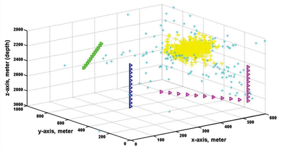
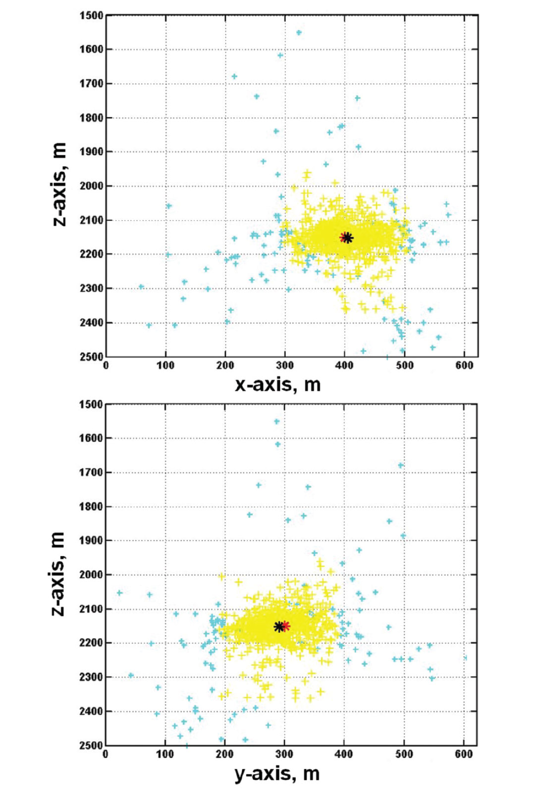
Figure 12 shows in 3D all the points of nearest approach in cyan and yellow. After two iterations of statistical clustering, all the cyan points are rejected as extreme outliers, and only the yellow points remain. The point with mean coordinates and the source point are hidden in the cloud of yellow points. Figure 13 show projections of the points on the x-z and y-z planes. On these displays, the source location estimated from statistical clustering is shown in black, while the true source point is shown as a red star. It can be seen that the estimated source location is very close to the true location, even though the initial propagation vectors (Figure 11c) appear to be totally random. The standard deviations of the coordinates for all the yellow points on Figure 13 are measures of the expected uncertainty in the estimated hypocenter location.
The example on Figures 11 to 13 is for the case of back-projecting through a homogeneous velocity structure. The extension to a layered-earth velocity structure is straightforward, and requires only the calculation of points of nearest approach for raypaths consisting of piece-wise straight lines.
Synthetic Files for a Swarm of Hypocenters
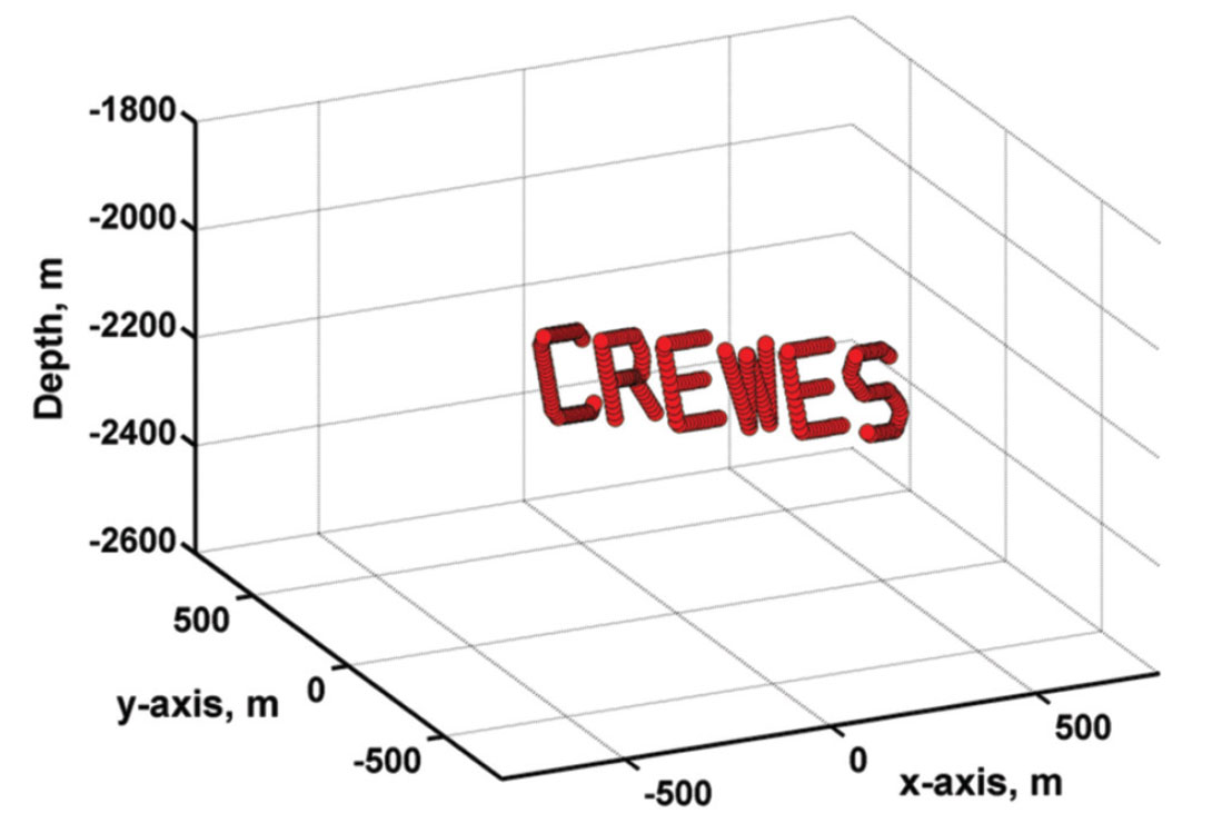
Since we are dealing with synthetic data, we can define microseismic sources anywhere in 3D space, with any recording geometry and any horizontally-layered velocity structure. For purposes of testing, we should generate files of synthetic microseismograms that correspond to a swarm of hypocenters with an easily recognized spatial distribution. Such a swarm is shown on Figure 14. When noise-free files corresponding to these hypocenters are given appropriate time stamps, location analysis of the synthetic data in sequence will give an evolving pattern of source points that spells out the word “CREWES”. Separate suites of files for the same swarm of source points and the same recording configuration, but with increased noise levels and with assumed uncertainties in the velocity structure, should provide data suitable for testing the effectiveness of particular location algorithms and processing flows.
Conclusion
Synthetic three–component microseismograms can be created by using ray-tracing or time-stepping finite difference (FD) modeling in horizontally-layered velocity structures. For the raytracing results, the modeled seismograms include only direct and head-wave arrivals, and the velocity model can include VTI or TTI anisotropy in the layers. The traces from FD modeling include reflected/converted as well as direct and head wave arrivals, but they do not include effects due to anisotropy. Gaussian and/or harmonic noise can be added to the synthetic microseismograms to simulate different signal-to-noise levels. The modeled data are stored in files with SEG-2 format to conform tofield-recorded data files.
These synthetic microseismic data files can be used for evaluating the effectiveness of various hypocenter location procedures for different recording configurations within hypothetical but realistic geological structures. Prior to drilling of observation wells for a proposed multistage hydraulic fracturing project, insight regarding the resolution capabilities of various recording configurations for hypocenter location can be gained by generating and analyzing synthetic data. Therefore, they are helpful for pre-survey design of optimal recording configurations. Synthetic P and S amplitudes generated by FD modeling should also give quantitative predictions of signal-to-noise ratios in velocity media where seismic shadow zones are expected to exist. However, FD modeling for computing synthetic seismograms is much slower than the ray-tracing method.

Acknowledgements
This research was supported by the NSERC and the industrial sponsors of CREWES. We thank Jamie Rich of Devon Energy Corporation for providing the velocity-density model shown on Figure 1.
Related Reading


Join the Conversation
Interested in starting, or contributing to a conversation about an article or issue of the RECORDER? Join our CSEG LinkedIn Group.
Share This Article