Introduction
Sander Geophysics’ AIRGrav airborne gravity project started in 1992 with the purpose of designing an airborne gravimeter that would be well suited to the dynamic environment of an aircraft. The five year research and development project resulted in the AIRGrav system, which has been used for airborne surveying since 1997. The majority of these surveys have been conducted for the petroleum industry, as well as some applications to mining exploration. At present, four AIRGrav systems are employed in worldwide survey operations in Sander Geophysics airplanes and helicopters.
The AIRGRav system
The AIRGrav system consists of a three-axis gyro stabilized inertial platform with three orthogonal accelerometers. Unlike older gravimeters, the AIRGrav system does not use any spring-type apparatus. The accelerometer is held within 10 arc seconds (0.0028 degrees) of level by a Schuler tuned inertial platform, monitored through the complex interaction of gyroscopes and accelerometers. This arrangement ensures that the gravimeter remains oriented vertically, independent of the manoeuvres of the aircraft.
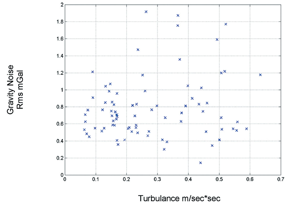
The three-axis stabilized platform used in AIRGrav is controlled in a fundamentally different way to the platforms used with the Lacoste and Romberg (L&R) or Bell gravimeters. The L&R and Bell two-axis platforms rely on a control loop which attempts to null the horizontal accelerometers on the platform with a settable time constant. The control loop used in AIRGrav relies on the very low drift of its high-accuracy gyros. This allows draped surveys to be flown and allows surveying in turbulence similar to what is practical for high resolution magnetometer surveys. This is demonstrated in Figure 1, which shows there is little correlation between noise level and turbulence.
The gravity sensor used in AIRGrav is a very accurate three-axis accelerometer with a wide dynamic range. This avoids the saturation that occurs with other systems during strong vertical motion of the aircraft. Testing has shown the accuracy of gravity recovery to be almost completely unaffected by aircraft dynamics up to what is considered “moderate” turbulence. The wide dynamic range also allows draped surveys to be flown, something which is nearly impossible with other gravimeters. The AIRGrav sensor has extremely low cross-coupling (i.e., errors introduced by deformation of the sensor and conversion of horizontal acceleration into vertical acceleration) due to the very tight servo control of its proof mass, and needs no corrections for this effect. The sensor is extremely linear and does not need a test range to be calibrated. The design of the platform is such that the sensor can be “tumbled” in the gravity field at a calibrated point to set the scale factor and offset.
AIRGRav operations
The AIRGrav system itself is lightweight, with an installed weight of less than 100 kg. This allows it to be installed in survey aircraft in conjunction with other geophysical equipment, including that necessary for magnetic surveys. The gravimeter has been flown in a range of aircraft; twin engine Cessna 404 and Britten-Norman Islanders, single turbine engine Cessna 208B Grand Caravans, as well as in a Eurocopter AS 350 helicopter. The resolution and accuracy of the final gravity data is primarily dependent on flying speed and line spacing rather than the type of aircraft. There are no additional restrictions on flight parameters beyond those typically used for aeromagnetic surveys in terms of operating altitude, ground clearance, and turbulence. Level flight is not required; a draped surface can be used to follow the terrain. Typically, a short lead-in of 3-5 km is flown to minimize online effects from aircraft turns. In practice, a large portion of this extension data can be included in the final data set because turn effects are minimal. The system has been used successfully offshore, in mountainous terrain, in deserts in Africa and the Middle East, and in the Canadian high arctic in winter conditions.
During field operations, the accelerometer scale factors and offsets can be calibrated at the survey base to correct for slow time variations in these parameters by rotating the platform through 180 degrees to measure the strength of the gravity of the Earth with positive and negative polarity. A test calibration range is not needed. The value used for gravity during calibration is ideally from a ground instrument or a known local gravity point, although it is possible to determine a local gravity value with sufficient accuracy using only the AIRGrav instrument. The system also automatically aligns and calibrates its gyros on start up before each flight, by determining the gyro drifts and XY bias.
Before and after each flight, the accuracy of the local gravity reading computed by the system is verified and instrument drift monitored by measuring gravity on the ground for 15 minutes or more. This period can also be used as an initialization period when the differential GPS data processing is performed, resulting in better accuracy. Daily before-flight and after-flight average readings are plotted and monitored for signs of instrument drift. Linear drift corrections have proved unnecessary and are not applied. Pre- and post-flight readings typically match within +/- 1 mGal, and variations over the course of a survey are only a few mGal.
Data processing
During survey operations, accelerations in an aircraft can reach 1 m/s, equivalent to 100 000 mGal. Data processing must extract gravity data from this very dynamic environment. This is achieved by modelling the movements of the aircraft in flight by extremely accurate GPS measurements. Dual frequency GPS receivers are employed on the aircraft and in ground reference stations used for differential GPS processing.
Extensive research at SGL has resulted in high quality differential GPS processing techniques which are critical to achieving high resolution and high accuracy gravity data. In addition to providing the lowest possible noise levels, these techniques allow surveys to be completed successfully despite poor satellite geometry and high ionospheric activity, an essential requirement for surveys in far northern and southern latitudes.
Gravimeter data are recorded at 128 Hz. Accelerations are filtered and decimated to match the GPS, recorded at 10 Hz, using specially designed filters to avoid biasing the data. Gravity is calculated by subtracting the GPS derived accelerations from the measured accelerations. The calculated gravity is corrected for the Eötvös effect and normal gravity, and the sample interval is reduced to 2 Hz.
Terrain corrections are computed using 2D FFT methods with a density appropriate for the area. Since the accuracy of the terrain correction is limited by the accuracy of the input terrain model, an on-board laser altimeter or LIDAR is employed which, in conjunction with differential GPS processing, enables the calculation of a digital terrain model in the survey area. As in ground surveys, poorly modelled terrain data could cause a significant error in the processed gravity data.
The gravity data are filtered to remove noise using a low pass FFT filter prior to free air correction. Different filter settings are used depending on the application. After the standard corrections have been applied, the gravity data are gridded using the same minimum curvature gridding algorithm that is used for aeromagnetic data. A 2D spatial filter is then applied to the gridded data to maximize the resolution of the data by allowing noise cancellation between adjacent lines.
Turner Valley case study
In 2001, SGL flew a large AIRGrav survey in Western Canada over the Turner Valley area, an oil and gas producing region south of Calgary, Alberta (Pierce et al., 2002a, b; Sander et al., 2002). The survey area covered the foothills of the Rocky Mountains. The general trend of the geology in the area is north-north-west / south-south-east. A total of 12 500 line km of AIRGrav and magnetometer data were acquired simultaneously using a fixed-wing aircraft. The survey was completed in less than five weeks over very mountainous terrain, ranging from approximately 1000 m ASL to approximately 2000 m ASL.
East-west traverse lines were spaced at 250 m and north-south tie lines at 1000 m.
Figure 2 shows the AIRGrav and aeromagnetic data acquired during the Turner Valley Survey. The colour image displays the first vertical derivative of Bouguer gravity, with the warm colours representing vertical gravity gradient highs. The grey shades are the shadow of the first vertical derivative of the aeromagnetic data.
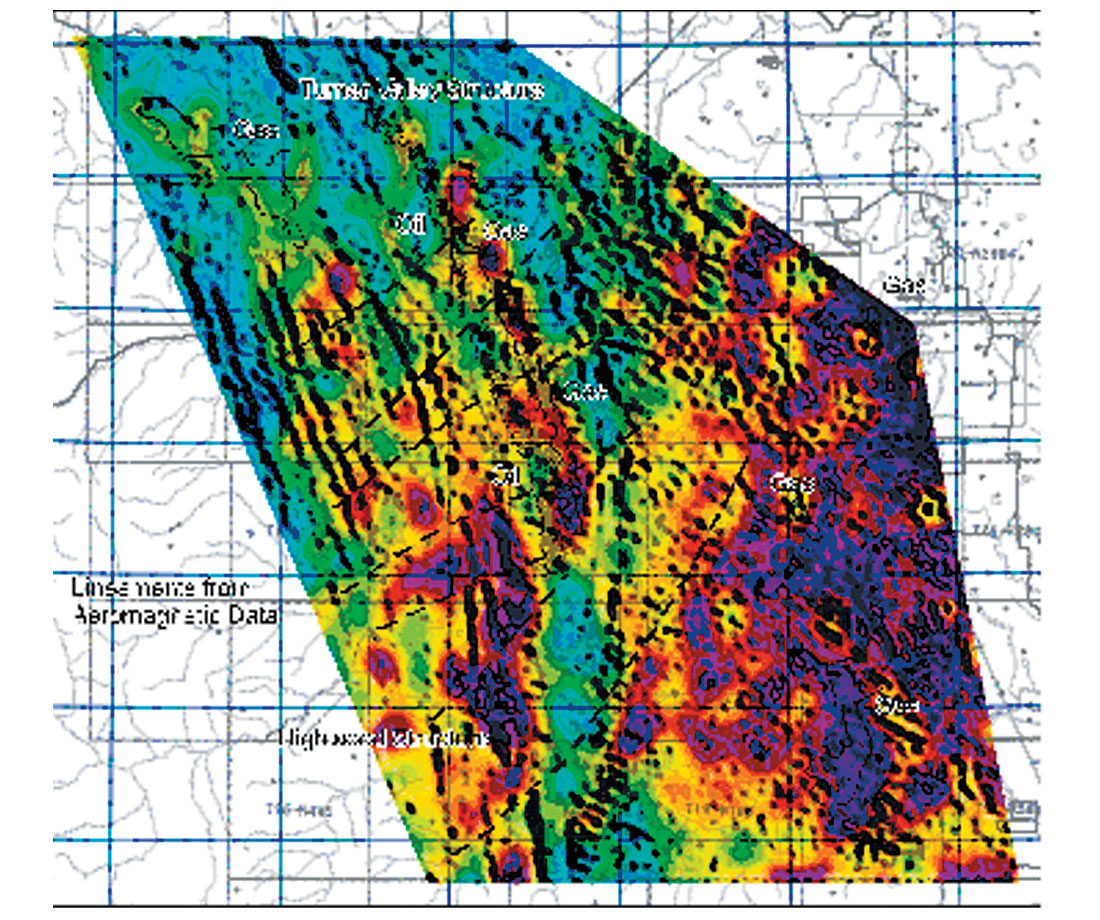
The western side of the survey area is dominated by north-south trending faults associated with the foothills region. The eastern side of the area consists of flat lying sediments. Gas and oil producing areas are outlined by solid and dotted lines respectively. The long northsouth trending field in the centre of the area is the Turner Valley Field, discovered in 1914. The Turner Valley and Quirk Creek Fields (in the north-west of the area) are generally associated with gravity highs. East-west trending lineaments, marked with dashed lines, were defined by joining terminations seen in the aeromagnetic data. The same lineaments also mark changes in the gravity signal, and offset the Turner Valley Field.
Existing ground gravity readings were compared with the AIRGrav data. Figure 3 shows the very good agreement between the two data sets. The uniform sampling provided by the airborne survey, however, brings out additional detail in areas that are sparsely sampled by ground data. Creating a grid of airborne gravity using only points where ground gravity exists improves the apparent correlation with the ground data, an indication that differences are due to improved airborne sampling (Pierce, 2002). The ability to provide uniform sampling over difficult terrain that is often inaccessible to ground surveys is one of the advantages of an airborne survey. The AIRGrav system is particularly well suited to this task it has low sensitivity to aircraft motion. The survey area is subject to frequent periods of turbulence caused by winds blowing down from the Rocky Mountains, and the climb into the foothills required a draped flying surface.
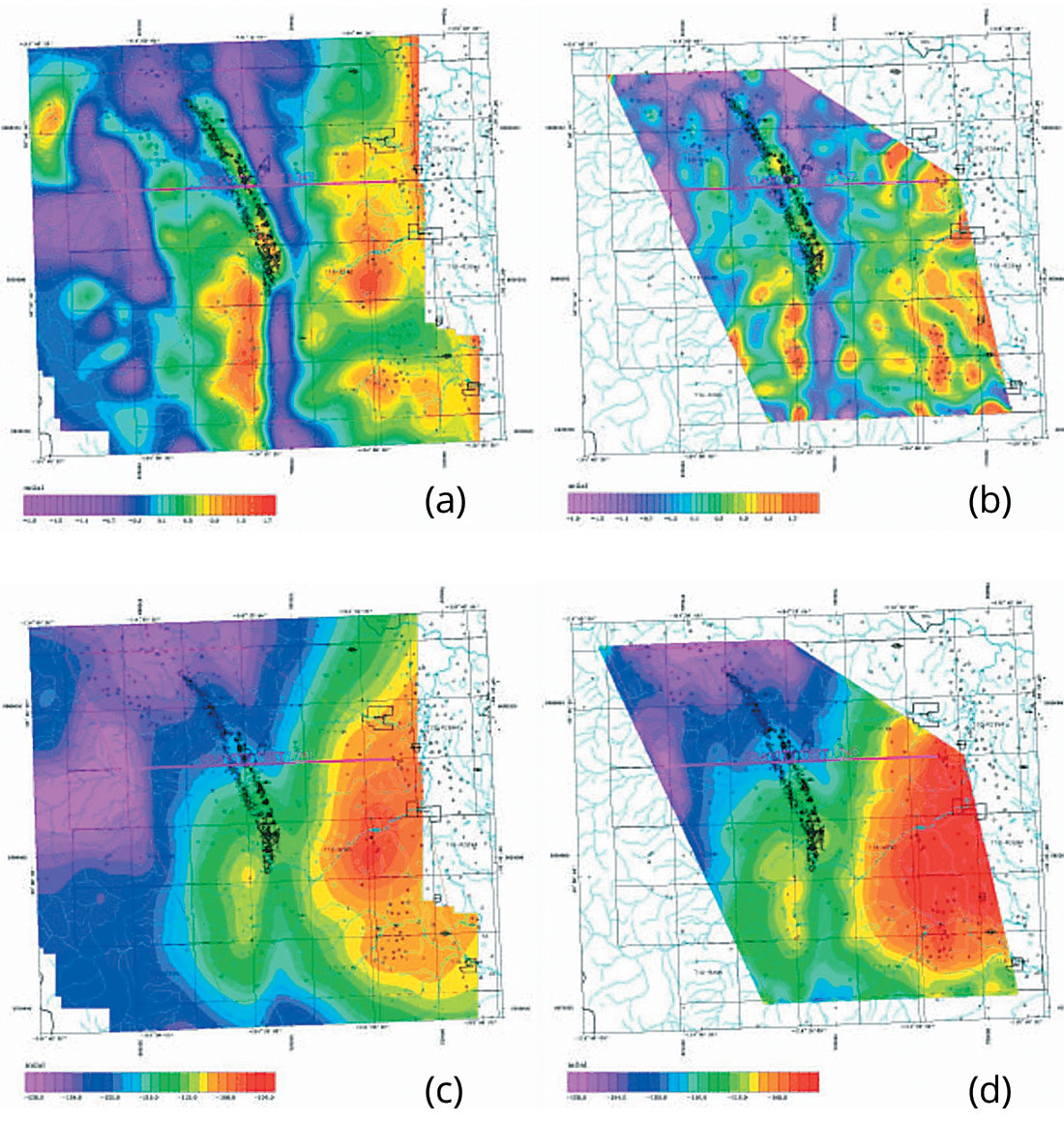
The images in Figure 3 (c) and (d) show the complete Bouguer gravity data, while (a) and (b) show the first vertical derivative of the complete Bouguer gravity data. The regional slope reflects the isostatic effect of the Rock Mountains, just west of the survey area. Figures reproduced from Peirce et al. (2002b).
Estimate of noise
Noise levels and system resolution require careful specification. Survey parameters, along with the instrument itself, are important factors in the resolution and accuracy of the final data products delivered to a client. A survey flown with tight line spacing, for example, takes advantage of over-sampling to reduce noise levels (Sander et al., 2003). Flying speed plays a role in determining AIRGrav resolution since the primary source of noise is from the GPS signal, which is time dependant. It is possible to increase the resolution to a degree simply by flying slower.
AIRGrav typically delivers gravity data which have been low-converted to wavelength. This equals a half-width of 2.0 km in a Cessna Grand Caravan or Britten-Norman Islander flown at 100 knots, 2.9 km in a Cessna 404 flown at 140 knots, and 1.0 km in a Eurocopter AS350 helicopter flown at 50 knots. Once the objectives of the survey are established, line spacing and flying speed are tailored towards meeting those objectives. In a recent petroleum survey flown in the Middle East, for example, 500 m line spacing was used. The final grid had real anomalies as small as 0.2 mGal and 2.0 km in size that were independently verified in a blind test using detailed ground measurements. Noise levels on the final grid data were 0.2 mGal, based on a measurement of internal consistency made using independent grids formed from alternate lines. This method of comparing independent grids of airborne data to estimate the precision of the measurements was applied in the Turner Valley example (Sander et al., 2002). The line spacing of 250 m over-sampled the data, given the application of a low-pass filter with 4 km cut-off. Two independent grids were produced by separating the data into two subsets (i.e., odd and even line number grids with 500 m line spacing). The rms value of the differences between these grids indicated a precision of 0.3 mGal for the complete dataset.
A case study for a survey in Timmins (Ontario, Canada) (Elieff, 2003; Elieff et al., 2004) quantified noise levels using a number of internal and external measures. This survey was flown with 500 m line spacing, and the gridded data were low-pass filtered with a cutoff wavelength of 2.85 km. The standard deviation of differences at flight and tie line crossovers indicated a precision of 0.45 mGal for the filtered line data. Differences between odd and even flight line number grids had a standard deviation that indicated a precision of 0.15 mGal in the final grid after spatial filtering. The standard deviation of differences between the airborne data and upward continued ground data was 0.62 mGal. This provides an upper bound estimate of the external accuracy of the system since it also includes errors present in the ground data and differences resulting from application of filtering to the airborne dataset but not to the ground dataset.
Conclusions
AIRGrav has been used to acquire airborne gravity data for both on-shore and off-shore surveys. The system allows drape surveys to be flown, resulting in better signal levels in survey areas with significant topographic relief. Final grids created with low-pass filters in the 2 – 4 km range have noise standard deviations between 0.15 and 0.3 mGal. This number is dependant upon survey parameters, such as line spacing and aircraft speed, as well as the details of the specific filter used.


Join the Conversation
Interested in starting, or contributing to a conversation about an article or issue of the RECORDER? Join our CSEG LinkedIn Group.
Share This Article