Introduction
Seismic acquisition is frequently being conducted in areas with extensive infrastructure as well as numerous environmental restrictions. Although some restrictions to seismic acquisition affect both sources and receivers, receivers are generally unencumbered due to their relatively small environmental footprint and ease of deployment. Accordingly, receiver infill stations can be used in place of source stations or in conjunction with source repositioning in order to mitigate the effects of a restriction. New cabled and cable-free technologies make the implementation of receiver infill stations easier and increasingly more cost effective and, as a result, their use is becoming more common place within the seismic data acquisition industry. The benefits of receiver infill stations are presented in the following case study based on a recently acquired 3D program in Southern Alberta.
Theory
A typical operational response when a surface source restriction is encountered is to reposition the source stations according to a defined set of source position guidelines. Source position guidelines are designed to mitigate the effect on trace distribution within the restriction while avoiding disruptions outside the restriction. There are several criteria for comparing trace distribution within or near a restriction including offset limited fold and azimuth/offset distribution.
Another approach, based on the theory of source-receiver reciprocity, is to use sources and receivers interchangeably when confronted with an acquisition restriction. Technical benefits of receiver infill stations stem from their ability to be deployed within areas where sources are restricted. By deploying receiver infill stations within the restriction fewer perturbations in trace distribution occur in the area surrounding the restriction. In addition, the offset/azimuth distribution within the restriction is improved relative to the use of source infill stations.
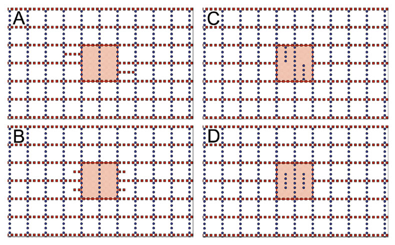
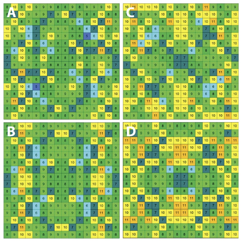
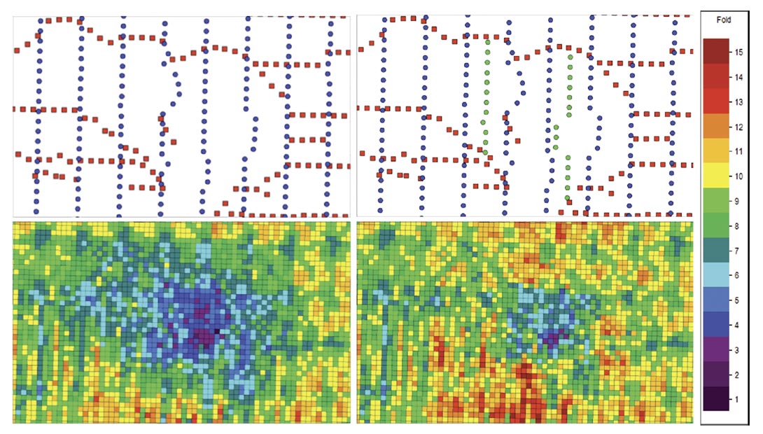
A theoretical comparison of repositioning sources versus receiver infill stations is illustrated in Figure 1. For simplicity, in these examples the source line interval is equal to the receiver line interval. A source restriction with dimensions that are twice the line interval is located within the center of the areas. In examples A and B the restriction is mitigated by following source positioning guidelines, with sources located outside of the restriction. In scenarios C and D the source stations are dropped and additional receiver infill stations are used within the restriction.
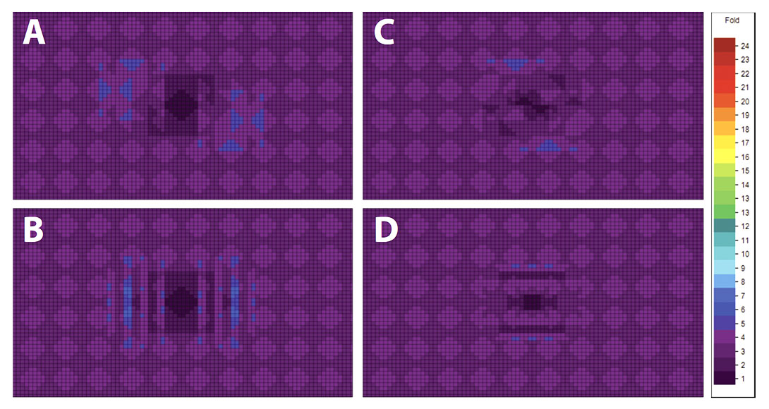
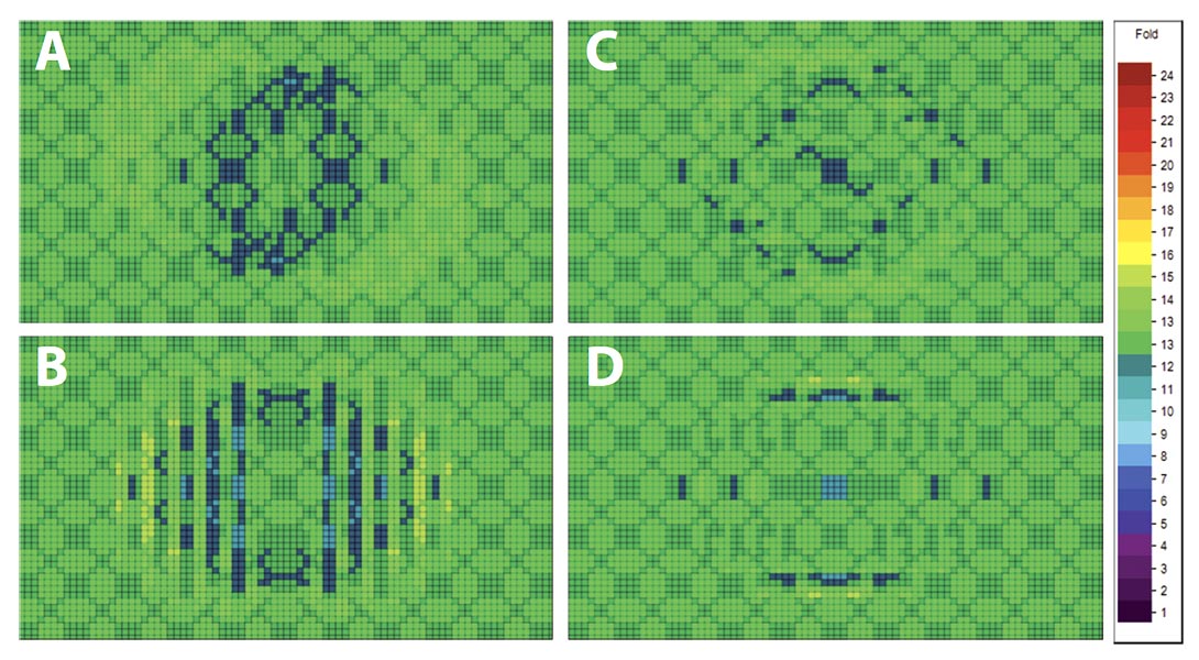
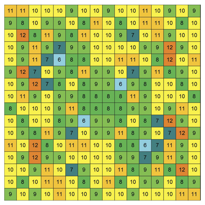
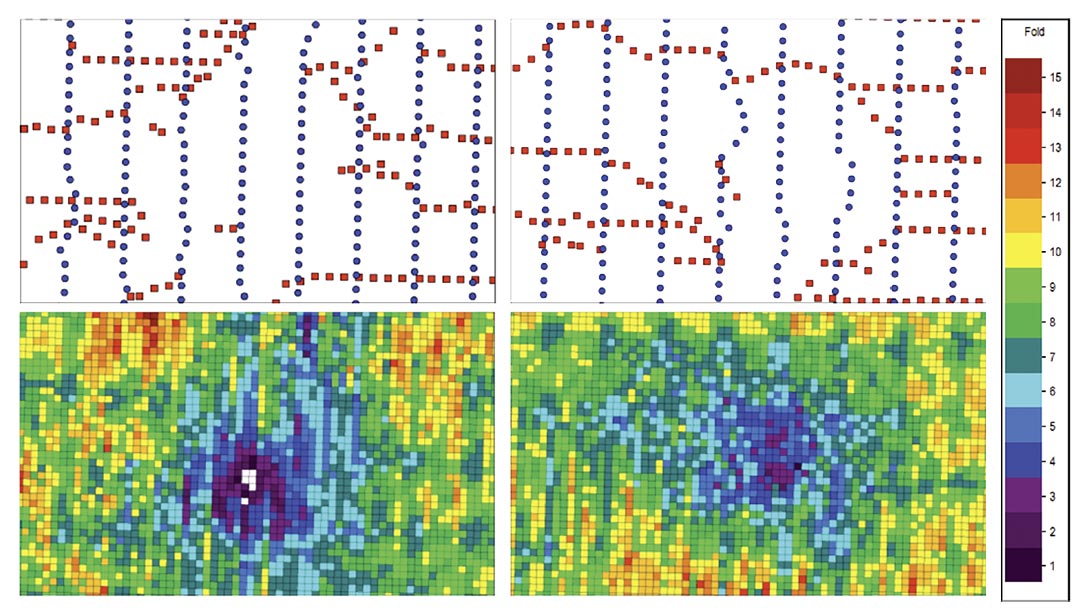
Offset limited fold plots for the four scenarios shown in Figure 1 illustrate differences in fold distribution depending on the location and type of infill station used (Fig. 2 & 3). Examination of the offset limited fold plots for near offsets (0-500m) and target offsets (0-1000m) indicate that receiver infill stations within the restriction result in less fold disturbance and an increased number of near offsets than repositioned sources.
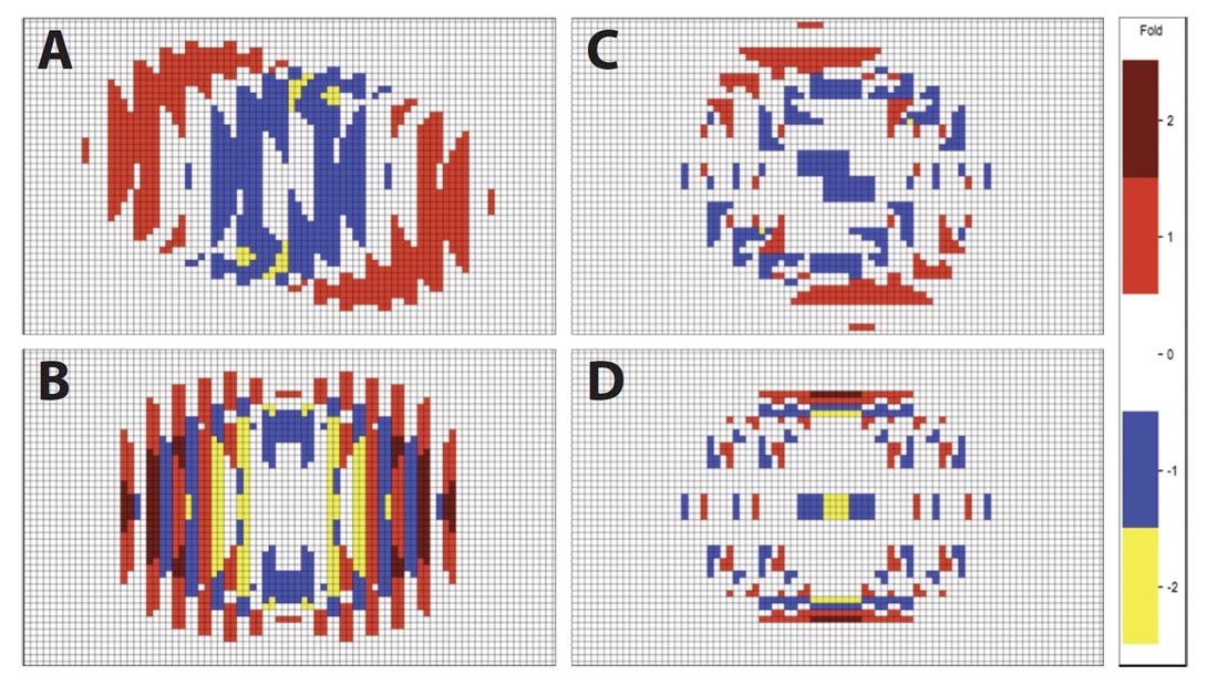
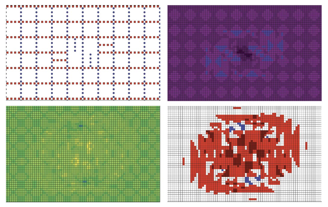
The resulting difference in fold from the theoretical distribution is shown in Figure 4. Bins with an increased fold contribution relative to theoretical are shown as red for +1 fold and dark red for +2 fold; bins with lower fold than theoretical are coloured blue for -1 fold and yellow for -2 fold; fold neutral bins are white. Both scenarios C and D, which use receiver infill stations, have a distinctly better distribution than scenarios A and B, which use source repositioning.
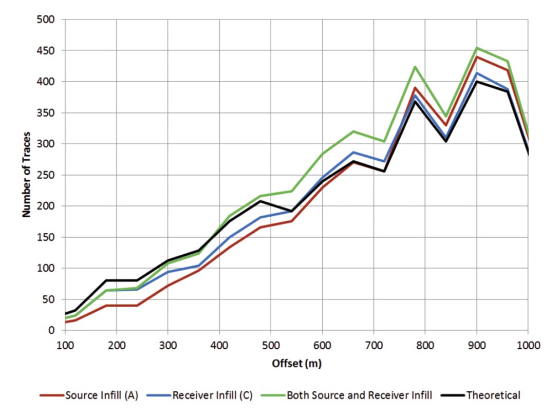
Although scenarios C and D minimize the impact of the restriction on fold distribution both within and around the restriction, there is an area of lower fold in the center of the restriction at a 0-1000m offset range. However, at an offset range of 0- 500m, receiver infill stations have a better fold contribution. Closer inspection reveals that most of the difference is due to fold from nonunique mid-offsets (Figure 5). Gathering traces in unique offset steps allows a direct comparison of the offset contribution from repositioning sources versus using receiver infill stations. Overall, receiver infill stations have a better unique fold distribution, whereas repositioning source stations produces a larger number of redundant offsets within the restriction. Figures 6 and 7 illustrate the effects of using both source repositioning and receiver infill stations. One way to reduce the number of redundant offsets while increasing the number of traces at the center of the restriction would be to use a limited amount of source repositioning along with the receiver infill stations. In general, bins within a restriction contain a higher number of traces with near offsets when receiver infill stations are used. This effect is illustrated in Figure 8 which compares the source infill from scenario A, receiver infill from scenario C, a combination of the two and theoretical.
Case Study Example: Explor Alberta Bakken 3D
The following case study demonstrates the effectiveness of using receiver infill stations to mitigate source restrictions. The Explor Alberta Bakken 3D was acquired by SAExploration in the fall of 2011 encompassing 481km² of land southwest of Lethbridge, Alberta. Parameters chosen to image the target were a source line interval of 300m, a receiver line interval of 240m, and a station interval of 60m for both sources and receivers. To acquire offsets of interest, a patch of 22 lines by 120 stations was recommended resulting in in-line offsets of 3600m and cross line offsets of 2640m. The parameters produce an average fold of 132 and a trace density of 146,667 traces/km² (Table 1). The program was acquired with a blended source of both Vibroseis and dynamite. Given the complex array of restrictions within the program and the operational efficiencies of a nodal (cableless) receiver, the decision was made to use a Fairfield Nodal ZLand receiver system.
| Program Parameters | |||
|---|---|---|---|
| Table 1: 3D Parameters | |||
| Source Line Interval | 300m | Receiver Line Interval | 240m |
| Source Station Interval | 60m | Source Station Interval | 60m |
| Patch | 22 Lines x 60 Stations | Offsets in Patch | 2640x3600m |
| Nominal Fold | 132 | Trace Density | 146,666 (traces/km²) |
Prior to the start of field operations, the theoretical parameters were remodeled using high resolution imagery and LiDAR 15 datasets to avoid known restrictions such as waterways, steep slopes and areas of operational difficulties. As a result of the pre-field modeling, the use of receiver infill lines to mitigate restrictions was planned prior to the start of data acquisition. During the field operations, seismic restrictions such as power lines, pipelines, and sensitive environmental areas were mapped by the survey company, and the applicable buffers/set-back distances were applied. This additional information was incorporated into the restriction model and further source repositioning and receiver infill stations were proposed.
Two areas with complex arrangements of restrictions that prevented deployment of sources in their theoretical location have been chosen for review (Fig. 9). Area 1 is located along the banks of the Milk River, with a 45m set-back from the high water mark, significant slopes, ferruginous hawk nests, springs, and other stakeholder considerations. Area 2 has pronounced development, with concrete structures, water wells, pipelines, and a wet, low-lying area that was in accessible for either type of source.
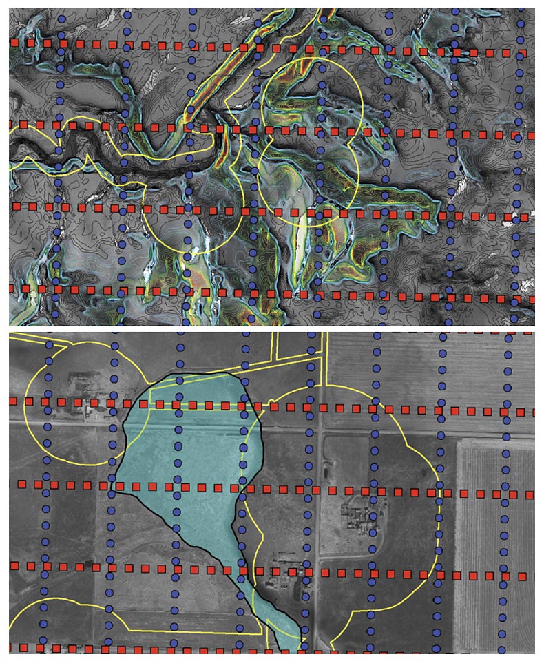
Through the application of source positioning guidelines, consultations with the client and iterative review of alternative station locations, a revised surface model was developed. The purpose of this model was to determine the effect the restrictions would have on trace distribution and maintain theoretical fold, azimuth, and offset distributions while minimizing disturbances. Despite optimal source repositioning, the large size of some restrictions resulted in lower fold than was acceptable, and in some cases (Area 1), resulted in several bins without any traces at offsets of interest (Fig. 10). In order to meet interpretive objectives, further effort was required to address the disparity from theoretical.
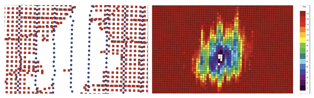
Since repositioned source stations already occupied a large percentage of the perimeter of these restrictions and sources could not be acquired any closer to the center of the restrictions, any additional sources around the perimeter were ineffective at contributing traces to bins that had zero fold. This is readily observed in Figure 11, which shows a model with all possible source locations surrounding the restriction in Area 1. Despite the additional effort, zero fold bins persist at the center of the restriction.
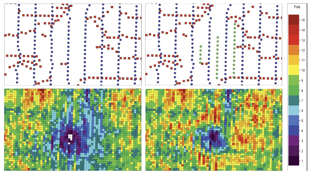
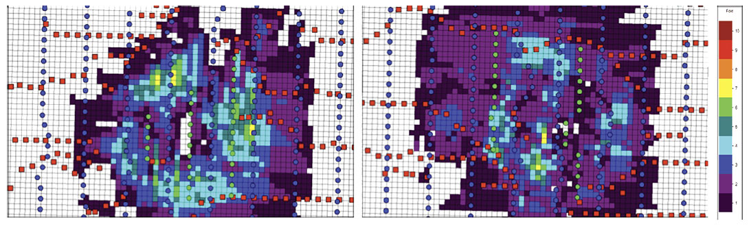
In order to mitigate the gaps in low fold areas observed in Figure 9, receiver infill stations were proposed and approved. Figures 12 and 13 illustrate the improvement in fold distribution obtained from the addition of receiver infill lines within Area 1 and Area 2. For operational reasons, deployment of the stations was parallel to the line orientation. Neither the restrictions nor the steep slopes along the river prevent receiver deployment, and the survey and recording crews could easily deploy the stations in the recommended locations.
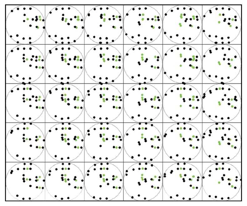
An analysis of the receiver infill stations highlights the improvement in trace density and illustrates the ability to fill previously empty bins. The additional fold due to receiver infill stations is shown in Figure 14. In some bins, the receiver infill stations contribute more than 8 fold. Offset and azimuth distribution is also improved. In Figure 15, receiver infill station contributions that provide a unique offset (gathered in discrete 60m segments) are coloured green and offsets from the conventional receiver lines are coloured black. Similarly, in Figure 16, green points within the polar azimuth plot represent contributions from infill receiver stations and black points represent contributions from the conventional receiver conventional receiver stations. (A polar azimuth plot displays the same information as a spider plot, but plots a point at the end of each vector.)

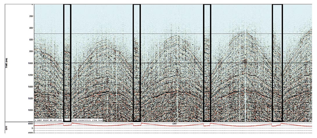
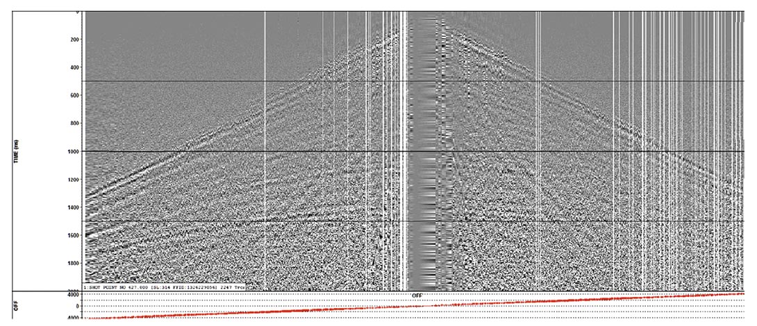
Meaningful data from receiver infill stations is readily identifiable on a subset of a shot record from the program (Fig. 17). The receiver infill traces are interposed between conventional lines and outlined by black rectangles. To better illustrate offset contributions of the receiver infill stations an offset sorted shot gather is shown is shown in Figure 18. Traces from receiver infill stations have been muted to highlight their position in signed offset. Observations conclude that there are many near offset contributions from the infill stations as well as a good selection of offsets on either side of the source.
Conclusion
As seismic programs are acquired in more developed areas with greater amounts of infrastructure, acquiring correctly sampled data becomes increasingly difficult. Even with optimal source repositioning around a restriction, gaps or low fold areas with a reduced offset/azimuth distribution can occur within a dataset. Receiver infill stations, however, can effectively mitigate these restrictions by filling empty bins, increasing trace density, and improving offset/azimuth distributions.

Acknowledgements
The authors would like to thank OptiSeis, Explor, SAExploration, Absolute Imaging, and AltaLIS for their contributions and consent to share this paper. This paper includes material © KARI 2011, Distribution Spot Image S.A., France, available from DigitalGlobe.
Related Reading


Join the Conversation
Interested in starting, or contributing to a conversation about an article or issue of the RECORDER? Join our CSEG LinkedIn Group.
Share This Article