Summary
In early September of 2011, CREWES (Consortium for Research in Elastic-Wave Exploration Seismology) collaborated with Husky Energy, Geokinetics, and INOVA, to conduct a seismic experiment designed to study the initiation and recording of very low frequency seismic reflections. The motivation was to collect a dataset that will be useful to test inversion methods. The site chosen was a 4.5km line, near Hussar, Alberta, that passes through 3 wells owned by Husky and near two others, all with good logging suites. Both dynamite and Vibroseis sources were tested along with 5 different receiver types. A specially modified low-frequency vibrator, the INOVA AHV-IV (model 364), was brought to the experiment by INOVA and a more conventional Failing (Y2400) was rented. Both vibrators were programmed with specially designed low-dwell sweeps which spend extra time in the low -frequency range. The receiver used were Vectorseis 3C (MEMS) accelerometers, 10Hz SM-7 (ION-Sensor) 3C geophones, 4.5Hz Sunfull 1C geophones, 10 Hz SM-24 highsensitivity geophones, and Nanometrics Trillium seismometers. The first 3 types were planted densely along the entire line while the last two were only available in limited quantities. A total of 12 P-P and 8 P-S lines were recorded and are presently being processed. Spectral analysis of raw records shows that in large part the various instruments performed as expected. There was significant low frequency energy excited by all four sources with dynamite being the strongest, followed by the INOVA 364 low-dwell, the Failing low-dwell, and the INOVA 364 linear, in order of the strength of low frequency energy. The Vectorseis receivers seem to record strongly down below 1 Hz; however the response is higher than the corresponding geophones. The 10 Hz SM-7 and 4.5 Hz geophones performed well down to their resonant frequencies. After application of the inverse filters for their instrument response, it appears that signal was recovered down to perhaps 1.5 Hz. We qualify these remarks with a cautionary note as these measurements are based on raw data not final processed images.
Introduction
In early September of 2011, CREWES (Consortium for Research in Elastic-Wave Exploration Seismology, a research project at the University of Calgary) collaborated with Husky Energy, Geokinetics, and INOVA to conduct a unique seismic experiment near Hussar Alberta. The goal of this experiment was to use modern source and receiver instrumentation to extend the seismic bandwidth as far into the low-frequency range as possible without sacrificing the higher frequencies.
A major driver for this research is the understanding that seismic inversion methods, both poststack impedance inversion and full-waveform inversion, require low-frequency information about the desired earth model. It has been common practice for many years to supply this lowfrequency information from well logs in the course of impedance inversion. While this has been a reasonable solution, well logs are usually only available at a few locations while seismic data is densely sampled spatially. If it were possible to get this information from seismic data, that would ultimately be preferable.
Most modern land seismic data are recorded with either 10 Hz geophones or MEMs accelerometers, with the former being the most common. The 10 Hz geophone performs very well in the band 10-250 Hz but below the 10Hz resonance, amplitude acceptable for many years and seismic signal bandwidths in final images, obtained on land, typically begin near 10 Hz. Now, with growing emphasis being placed on accurate inversion for rock properties, the 10 Hz low-end is becoming increasingly unsatisfactory. In truth, a 10 Hz geophone records data well below 10 Hz but its recovery requires applying an inverse filter for the geophone response (Bertram et al, 2011). From these observations a number of questions arise such as
- How low can 10 Hz geophone data be pushed?
- How low can MEMs accelerometer data be pushed?
- What are the issues related to geophones with lower resonance frequencies?
- What are the best seismic sources to generate low frequencies?
- How low must the bandwidth be pushed to see a significant benefit in inversion?
- Can low-frequency surface waves and reflection information be reliably separated?
Can the lowest frequencies be recorded with sparser spatial sampling than the conventional band? If so, how should the two recordings be merged?
We report here on the description and conduct of the Hussar experiment and present a few initial results from data analysis of the raw records. The answers to the above questions will require much more time and space than that available here. Elements of this work also appear in Archer et al. (2012).
Description of the experiment
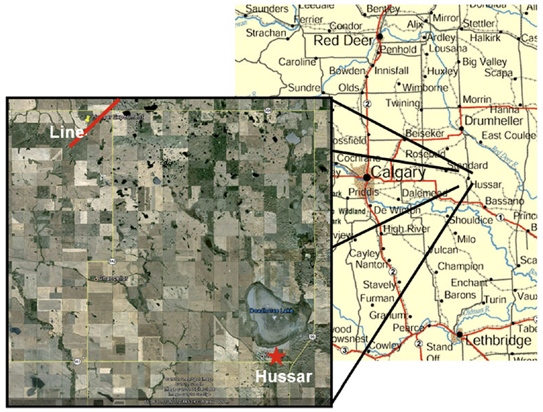
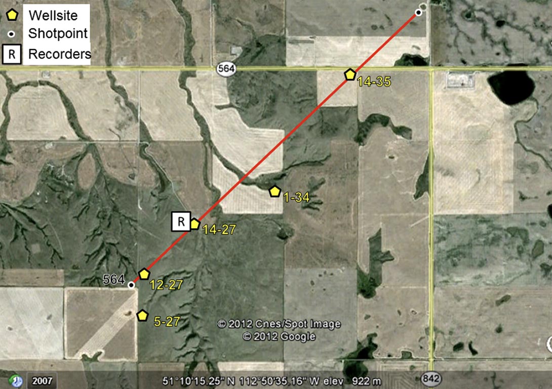
This experiment was designed by researchers at CREWES in consultation with geophysicists at Husky Energy, Geokinetics, and INOVA. A site near Hussar, Alberta (Figure 1) was chosen primarily because of easy access from Calgary and excellent nearby well control (Figure 2).
Husky Energy managed all apects of the survey including land access and subcontracting. INOVA mobilized one of their model 364 low-frequency vibrators from Houston just for this experiment. This vibrator has a specially designed and strengthened baseplate and other enhancements designed specifically to improve its low-frequency performance. Geokinetics supplied a professional seismic crew, recorder, and sufficient Vectorseis 3C MEMs accelerometers for the experiment.
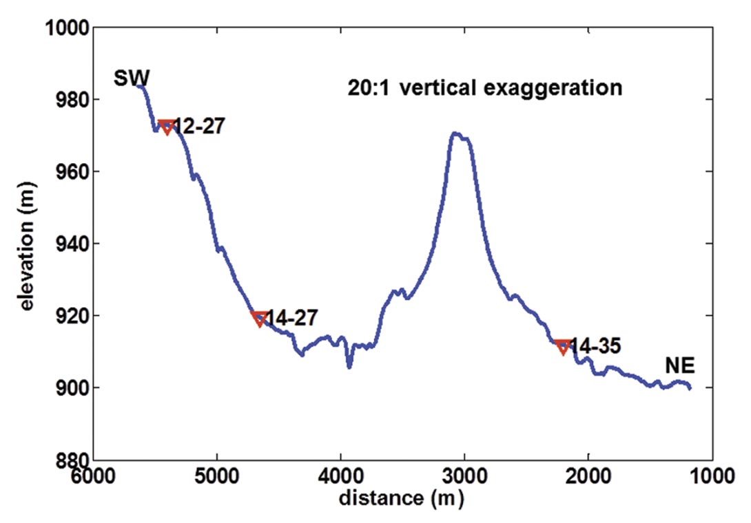
The line location (Figure 2) directly ties 3 wells (12-17, 14-27, and 14-35) while two more are nearby. All wells have p-wave sonics, density, and gamma ray logs while 12-27 has an s-wave sonic. The logs in 12-27 extend from 200m to 1600m depth. Initially the line was designed to be 6 km long to extend 1.5 km SW past well 12-27 (to the bottom left of Figure 2). However, we were unable to get land access and the line had to be terminated as shown with a final length of 4.5 km. Topographic variation along the line is significant (about 70m) but caused no major difficulties.
Receiver layout
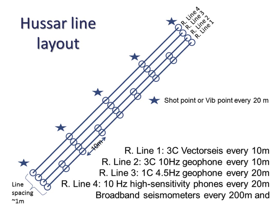
A wide variety of receivers was used and deployed in four separate lines, one meter apart as shown in Figure 4. The source locations are also indicated. The receiver spacing on lines 1 and 2 was 10 m while on line 3 it was 20 m. Line 1 was populated with 3C Vectorseis MEMs devices, line 2 had 3C 10Hz geophones, and line 3 had 1C 4.5 Hz geophones. All three lines were fully populated with receivers. Line 4 had a mixture of devices most notably 15 broadband Trillium seismometers deployed at 200 m intervals and 50 (ION-Sensor) high-sensitivity 1C geophones deployed at 20 m intervals around well 12-27.
While it would have been nice to have some 2 Hz geophones or perhaps 3C 4.5 Hz geophones, it proved impossible to obtain these in the available time frame. We are confident that the assortment of receivers used should allow us to push the bandwidth to the 1-2 Hz range. The seismometers should allow us to establish the actual signal at low frequencies for comparison with the other receivers.
Recording systems
Two different recording systems were used. ARAM/Aries recorded the 10 Hz and 4.5 Hz geophones and ION/Scorpion recorded the Vectorseis units. Both systems have built-in low-cut filters that were explicitly turned off for this experiment. At this time, there is some residual doubt about whether or not the ION/Scorpion lowcut filter was truly off but we can see no evidence of it in the spectra. The ARAM/Aries filter was definitely off.
Source effort
The source locations were all occupied 4 times so effectively there were 4 source lines and all the receivers were live for each shot. It is not clear from the outset what source configuration or type will prove most effective at low frequencies so we simply made some informed guesses.
Dynamite was the first and obvious choice and a blast is expected to approximate an impulse and hence radiate significant power at “all” frequencies. A common rule of thumb is that the larger the charge the lower the frequency. However, avoiding blow-outs requires larger charges to be buried at greater depths and this tends to move the ghost notch into the signal band. Previously at Blackfoot field in 1995, where the geology is very similar to Hussar, a 6kg charge placed at 18m depth was used (Gallant et al., 1995). Alternatively, current lines shot in the Hussar area by Husky tend to use a charge of 2kg at 15m. We decided to go with current practice and chose 2kg at 15m. Our decision was shaped by both economic concerns (e.g. the cost of dynamite and shot-hole drilling) and by the understanding that 2kg has produced sufficient bandwidth for exploration purposes in this area.
Vibroseis used at low frequencies is much more problematic than dynamite, but also potentially much more deterministic and controllable. The key limiting factors at low frequencies are the reaction mass stroke and the peak de-coupling force with the former being dominant at the lowest frequencies (Wei and Phillips, 2011). An additional limit of many vibrators is imposed by the total pump capacity and flow limitations of the servo valve and actuator combination (Lansley, 2012). Due primarily to the physical limits on reaction mass stroke, there is a 12db/octave ground force roll-off at low frequencies (Maxwell et al, 2010; Wei et al., 2010). As an additional concern is the fact that the far-field particle velocity is equal to the time-derivative of the ground force, causing an additional 6 db/octave loss (e.g Baeten et al, 2010). At CREWES, we have experience with our Envirovibe running at frequencies near 5 Hz and below (see Hall et al., 2010) and found that, even at greatly reduced power, the vibrator performs poorly. For example, a 5 Hz monochromatic sweep actually was found to radiate at many other frequencies with a dominant power near 15 Hz.
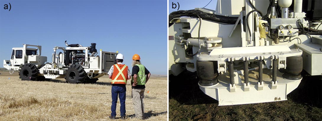
With these difficulties in mind, we approached INOVA with a request to support our experiment by allowing us to use their newly designed AHV-IV Commander (with a PLS-364) actuator low-frequency vibrator (described in Wei and Phillips, 2011). This vehicle (Figure 5) was specially built to radiate cleanly (i.e. with minimal distortion) at low frequencies. One of the important modifications is a specially stiffened baseplate (Figure 5b). INOVA generously agreed to help and mobilized an AHV-IV Commander (which we will hereafter refer to as the INOVA 364), with a 62,000 lb hold-down weight, directly from Houston specifically for our experiment.
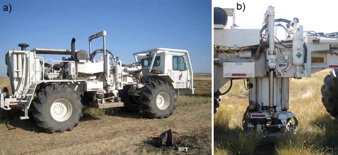
As a comparison vehicle, we also arranged, through partner Husky Energy, for a standard production vibrator, which was a 47,000 lb Failing (model Y-2400) vibrator (Figure 6).
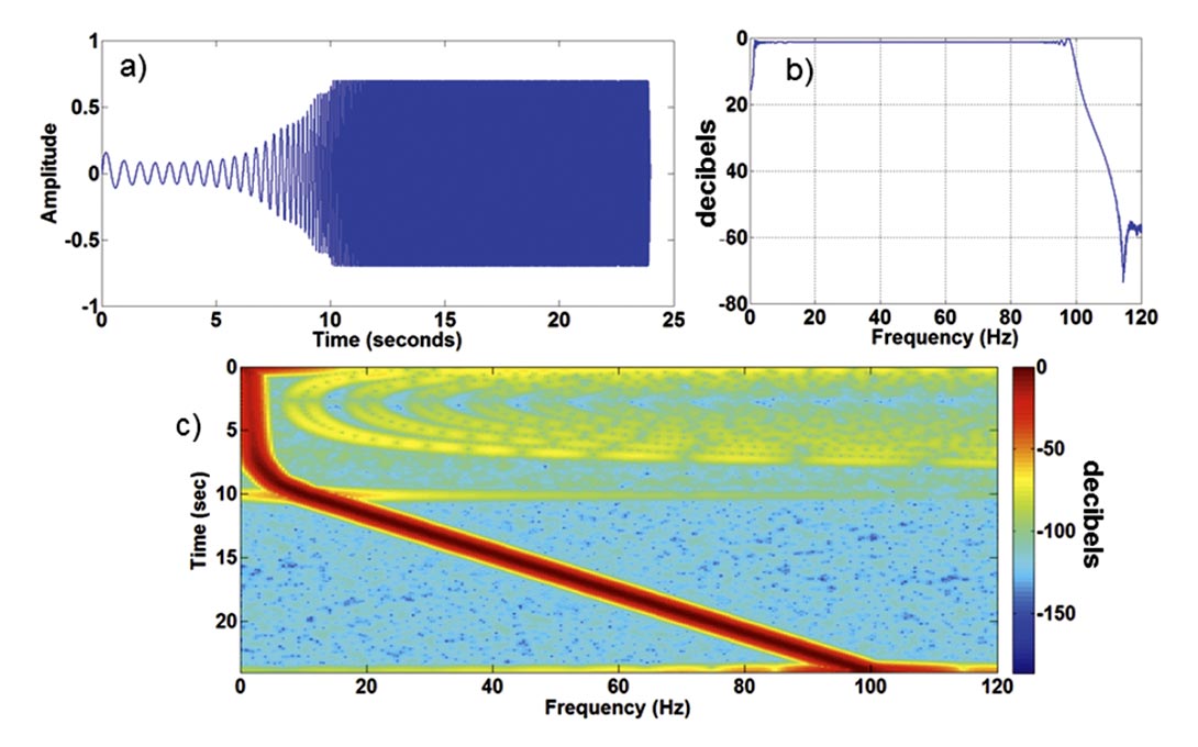
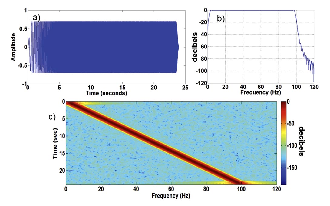
Sweep design becomes increasingly important at lower frequencies because the total sweep power must be reduced to avoid destructively large displacements of the reaction mass. We were aided in this by Tom Phillips of INOVA (Houston) who was present for the experiment and designed custom low-dwell sweeps for each vibrator. Figure 7 shows the low-dwell sweep used on the INOVA 364. In panel a) the sweep in the time domain can be seen to move slowly through the low frequencies at reduced power for the first 10 seconds, where normal linear sweeping begins at about 8 Hz. The reduced power is precisely compensated by the extended sweep time so that the Fourier amplitude spectrum (Figure 7b) of the sweep is essentially flat from 1 to 100 Hz. The Gabor spectrum of the sweep (Figure 7c) gives the complete story, showing a slow, linear trend from 1 to 7 Hz linked to a fast linear trend from 9 to 100 Hz. The sweep is designed to keep the INOVA 364 comfortably within its performance limits.
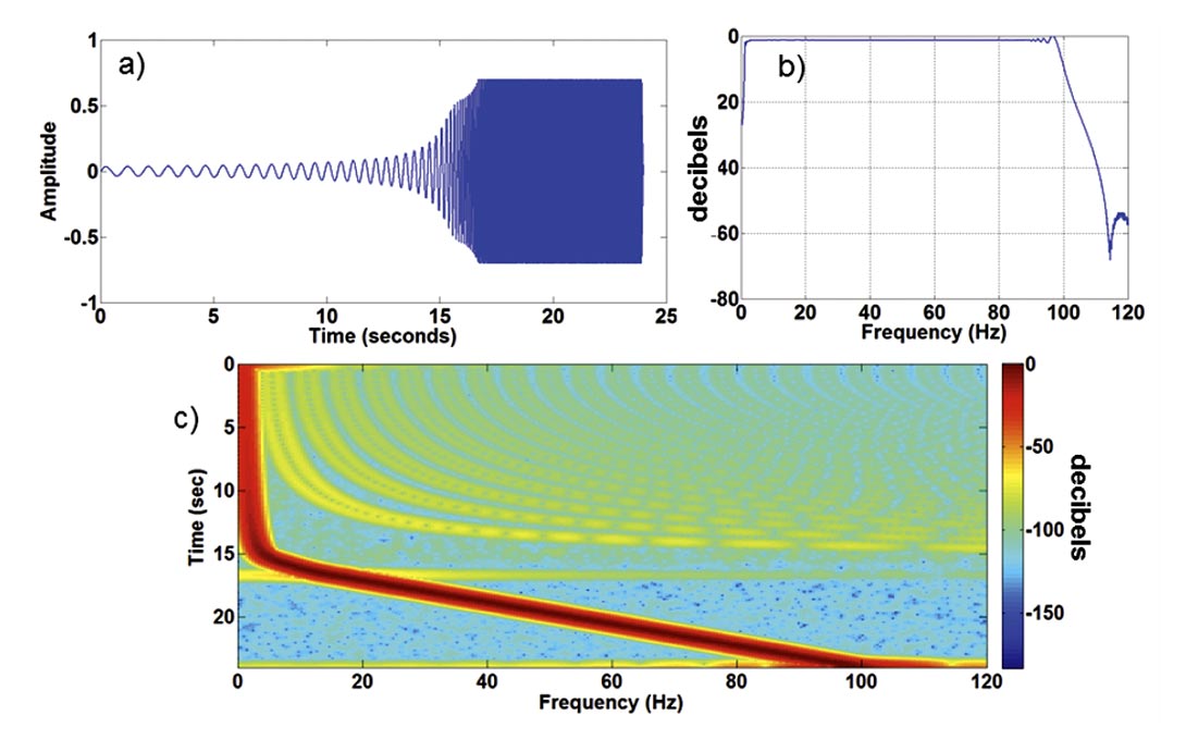
A similar low-dwell sweep was designed for the Failing Vibrator and is shown in Figure 8. The sweep shows a much longer lowdwell and a corresponding reduction in the time spent in the 8- 100 Hz range. For comparison, a standard linear sweep from 1 to 100Hz is shown in Figure 9. This sweep was also run on the INOVA 364. Figure 10 shows a true relative amplitude comparison of the three sweeps in the Fourier domain. It is apparent that the linear sweep shows greater overall power, a consequence of the fact that it spend more time over the conventional frequency range of 10-100 Hz. Also, all three sweeps had the same ½ second start and end tapers. The effects of these tapers are present in all of the spectral plots.
| Source | Interval | Parameters |
|---|---|---|
| Table 1: Summary of source effort at Hussar. | ||
| Dynamite | 20m | 2kg at 15m in a single hole |
| INOVA 364 | 20m | 1-100Hz low-dwell sweep (Figure 7) |
| INOVA 364 | 20m | 1-100Hz linear sweep (Figure 9) |
| Failing | 20m | 1-100Hz low-dwell sweep (Figure 8) |
| Dynamite | 3 locations | Test holes: 4kg @ 18m, 2kg @ 18m, 2kg @ 12m |
Table 1 shows a summary of the source effort. In addition to the sources discussed, there were also additional dynamite test holes at 3 locations along the line. Similarly, on the receiver side, receiver line 4 contains isolated special purpose instruments that are not sufficient in number to make a full section. In terms of complete lines, there were four separate source lines and three separate receiver lines (Figure 4). Since two of the receiver lines are 3C, we have the ability to make 12 PP sections and 8 PS sections.
Spectral Analysis of the Raw Data
We recorded both correlated and uncorrelated records and, considering only receiver lines 1-3, we have 4 sources recorded into each line. The resulting dataset is quite large, occupying roughly a terrabyte on disk (including the uncorrelated data).
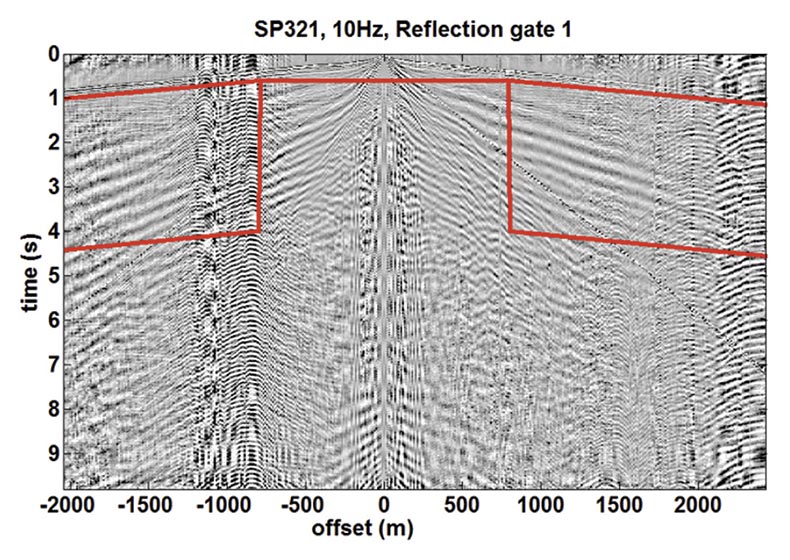
Here we show some interesting spectral analyses on a selected shot record. This is shot 321 which is located near the line center. An example of this record as recorded on 10 Hz geophones for the 364 low-dwell sweep is shown in Figure 11. Also show is the spectral analysis gate, which was chosen to avoid the near offsets and the first breaks while hopefully concentrating on reflected energy. The spectral analysis then computed the 1D spectrum of each trace in the analysis gate. Within the gate, each trace segment was multiplied by an analysis window whose width fluctuates randomly within a prescribed range. This fluctuating windowing technique reduces artifacts associated with the window geometry. Finally, we compute the average amplitude spectrum of all the windows in the analysis gate for comparison with other sources and receivers.
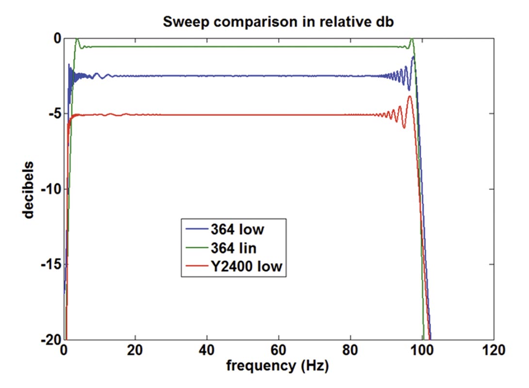
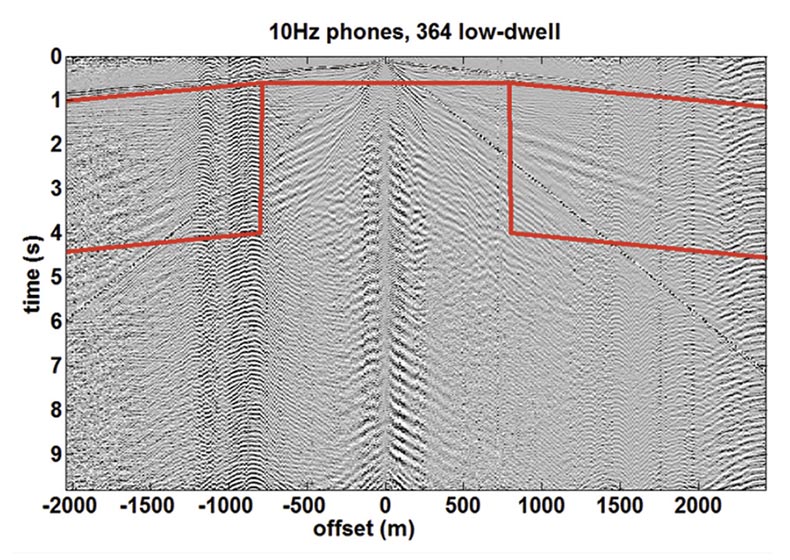
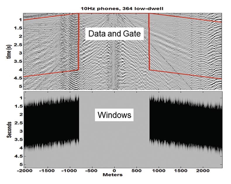
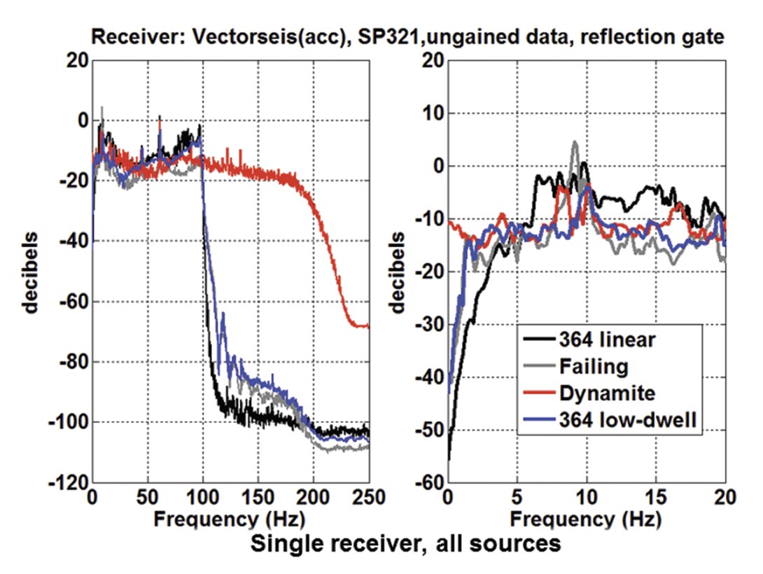
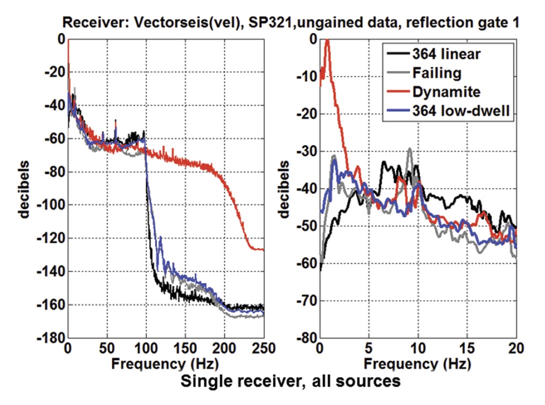
Figure 13 shows four average amplitude spectra, corresponding to the four different sources (Table 1) as recorded into the Vectorseis receivers. Since all data for a given receiver type was recorded by the same instrument in our experiment, it follows that we can compare the source types in true relative amplitude by holding the receiver type constant. We have done this and present decibel plots where the reference amplitude for all curves was the maximum value found on the dynamite spectrum. (The only possible problem with this idea is if the Vibroseis correlation was not properly normalized. However, the fact that the spectra track very close to one another is evidence that a normalized correlation was used in the field.) In Figure 13, the Vectorseis data is raw acceleration; but for direct comparison we convert to velocity as shown in Figure 14. Conversion requires an integration of the trace samples, which, in the frequency domain, is a division by i f (f is temporal frequency). The spectral trend as f → 0 in Figure 13 is essentially constant while in Figure 14 there is a strong increase consistent with multiplication with 1/f. Several observations can be made from these figures including:
- The linear vibroseis sweep shows less power at low frequencies than either low-dwell sweep. It drops off sharply around 4 Hz.
- The low-dwell sweeps show comparable amplitude levels that remain strong down to 2 Hz or perhaps lower.
- The dynamite shows a very strong low-frequency content especially in Figure 14.
These results are consistent with similar results from other locations on the line. We do not yet know if the low-frequency response seen on the dynamite data is indicative of reflection signal or not. The observation that reflectivity computed from well logs rolls off at the low frequencies argues that this is not reflection signal.
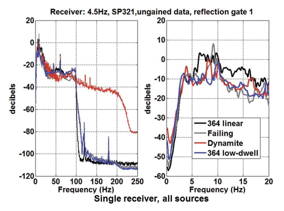
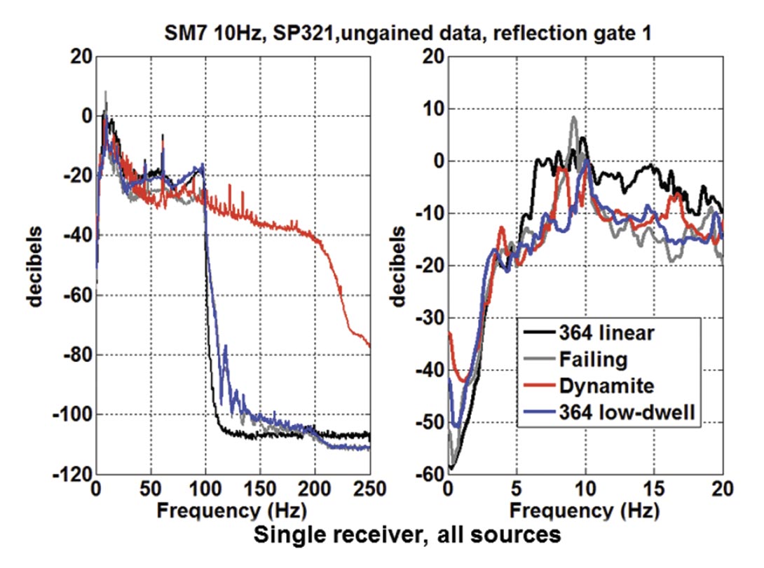
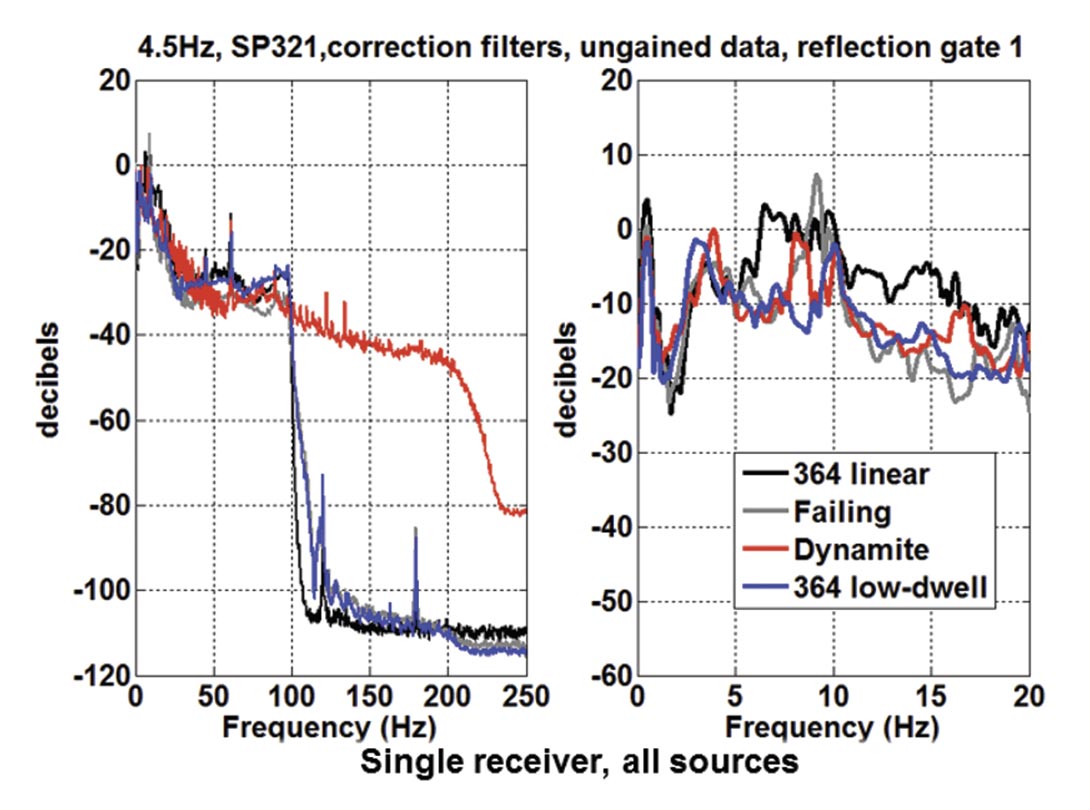
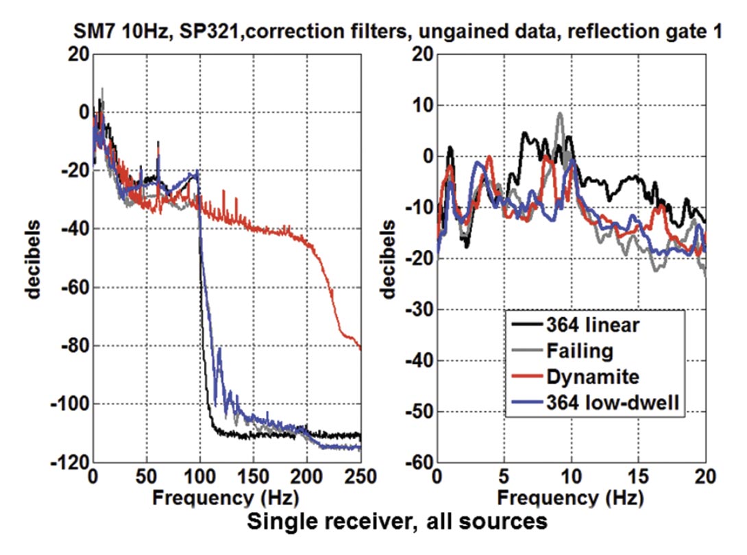
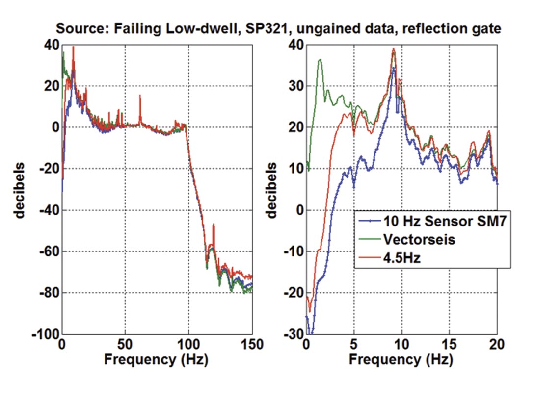
Figures 15 and 16 show the same shotpoint 321 as Figures 13-14 but now we examine the response of 4.5Hz Sunfull geophones and SM-7 (10 Hz, ION-Sensor) geophones. In Figure 15 the rolloff of the response below 4.5 Hz is clearly evident as is the similar but more severe roll-off of the 10Hz geophones on Figure 16. For either of these geophones the low-frequency response of our sources is not optimized. Bertram and Margrave (2011) showed that the geophone instrument response can be modelled as a Butterworth high-pass filter whose cut-off frequency is the characteristic frequency of the geophone. The geophone response can then be “corrected” by applying the inverse of the corresponding Butterworth filter. Numerically, we generated the impulse response of the corresponding Butterworth filter at the same length as the trace and divided the trace spectrum by the Butterworth spectrum in the frequency domain. This avoids any limitations that might be imposed by a temporally short inverse operator. The result of doing this for the 4.5Hz and 10Hz phones is shown in Figures 17 and 18. It might appear that frequencies below 1 Hz have been recovered by this process, but that is unlikely. Figure 19 is a repeat of Figure 11 except that the 10Hz geophone response has been corrected. As can be seen there is a considerable enhancement of low-frequency noise.
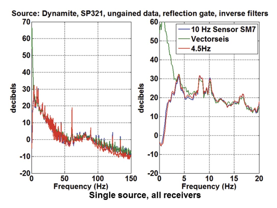
An alternative way to view the same information is to fix the source type and compare the receivers directly. However, this means that a true relative amplitude comparison is more difficult. As a simple alternative, we chose to normalize all of the amplitude spectra to their own value at 70 Hz, which means that their spectra will appear equal at this frequency. Figure 20 shows the response of the three receivers (Vectorseis, 4.5Hz Sunfull, and 10Hz SM-7 ION-Sensor) to the dynamite source at shotpoint 321. It is immediately apparent that the 10Hz spectrum begins trending down below about 9Hz, consistent with the geophone specs, and the 4.5Hz spectrum begins trending down (relative to the Vectorseis) at about 8Hz. If the Vectorseis spectrum is assumed correct, then we must conclude that the 4.5Hz geophones are not performing to specifications; however, we could also infer that the Vectorseis spectrum is trending anomalously upward. To further investigate this, in Figure 21 we show the same spectra but computed after the geophones have been corrected for their intrinsic low-frequency roll-off. Here we see the 4.5Hz and 10Hz responses have been essentially equalized while the Vectorseis is still showing an upward departure around 8 Hz.
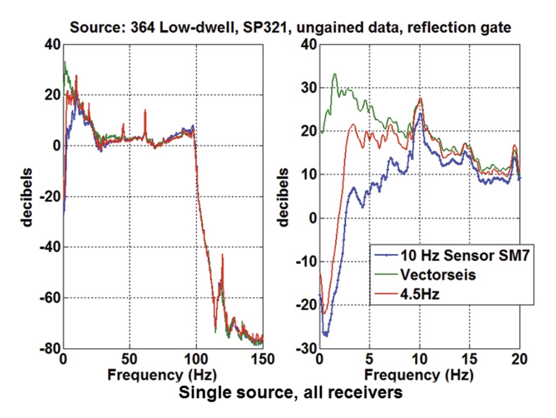
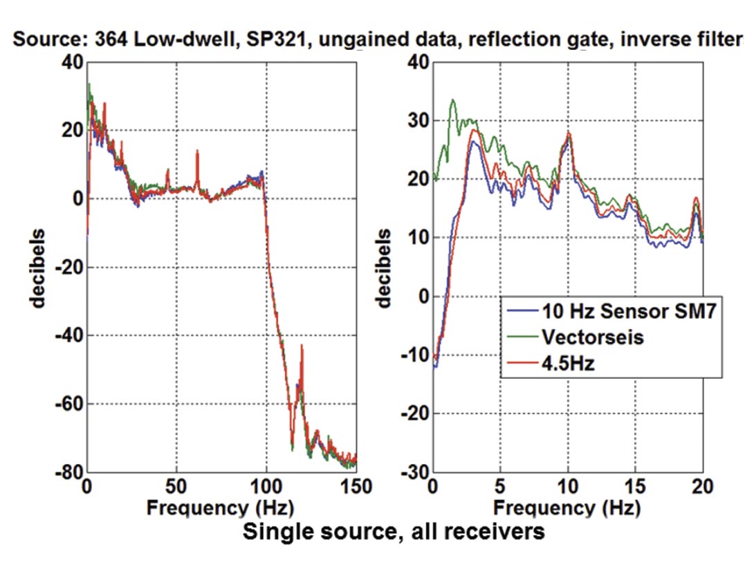
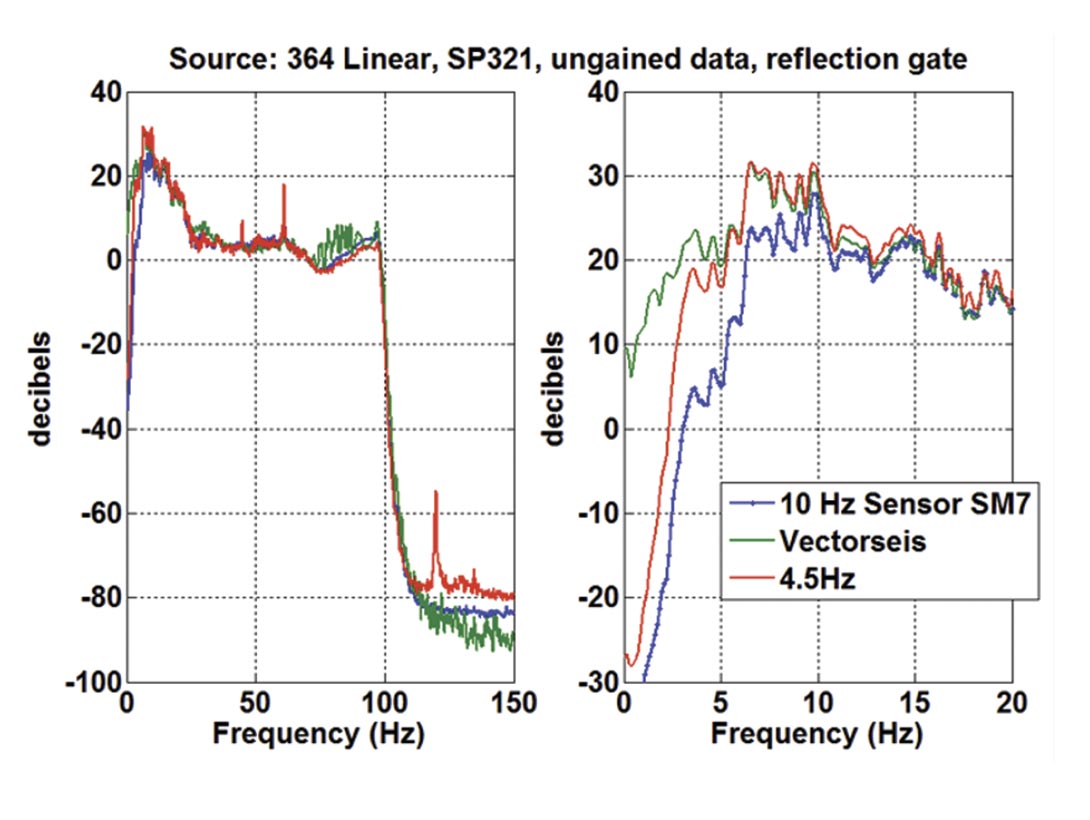
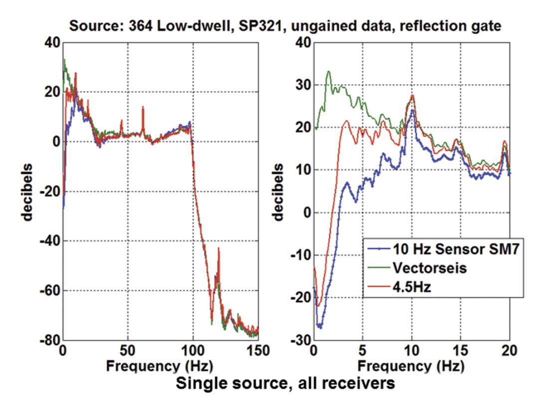
Figures 22 and 23 repeat this comparison for the 364 low-dwell sweep. The story on the low-end seems quite similar to before. In Figures 24 and 25 we show the receiver comparison for the 364 linear and the Failing low-dwell sweeps but we omit showing the geophone corrections. While we still see evidence of the Vectorseis upward trend, it does seem to be source dependent. The exact nature of this is uncertain. There is mention in the literature of 1/f noise in MEMS devices but this is usually considered to be an effect only below 1 Hz. If 1/f noise is the source of the upward trend seen here, then it seems to have significant effect at significantly higher frequencies. We note that the detailed features of the Vectorseis spectrum match those seen in the geophone spectra down to roughly 2-3 Hz.
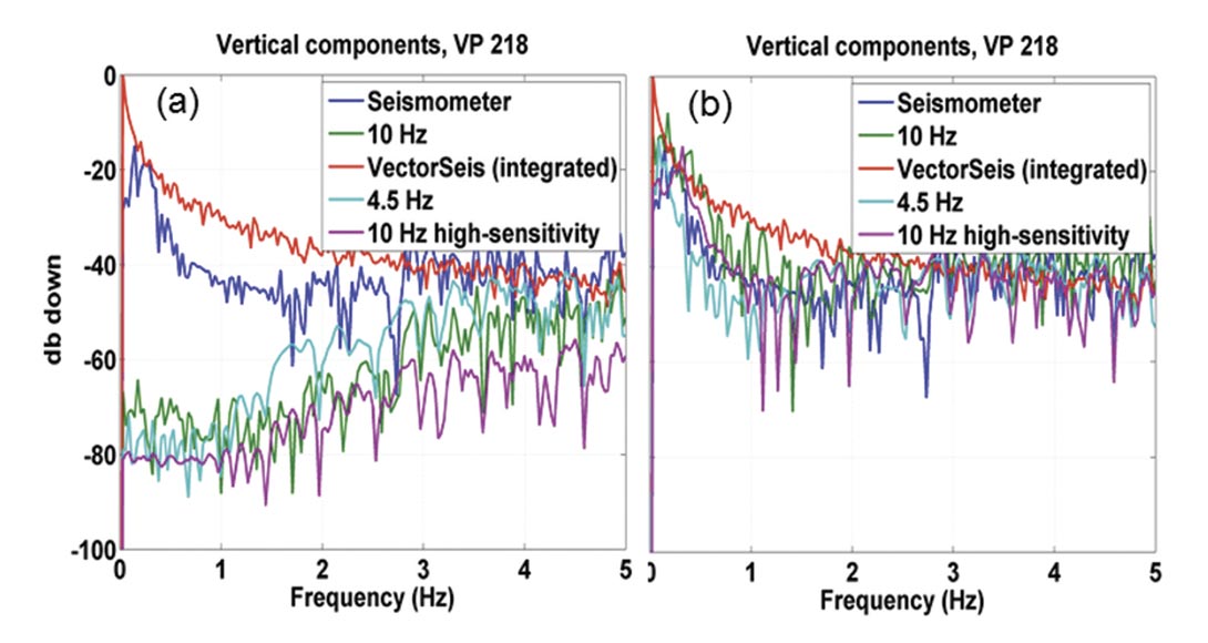
Another observation with bearing on this matter is shown in Figure 26. Here the spectra, for 0-5Hz, of the three industry receivers (Vectorseis, 4.5Hz geophone, 10 Hz geophone) are compared to a broadband seismometer, the Trillium manufactured by Nanometrics. The source in this case was an earthquake that occurred during the Hussar experiment (see Hall et al., 2012). Before the geophone corrections are applied, the geophone spectra trend below the seismometer and the Vectorseis is above. After applying the geophone correction, the geophones now have a trend matching the seismometer while Vectorseis is, of course, unaffected. Worth noting is that these spectra do not match well in detail, only in trend.
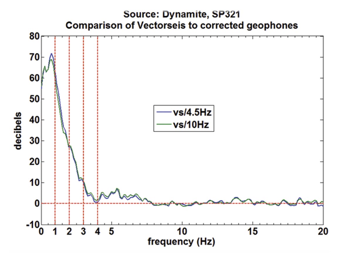
Finally, in Figure 27, we show the ratio of the Vectorseis spectrum of Figure 23 to the two geophone spectra of the same figure (these are the corrected geophone spectra). To produce these curves, a constant least-square scalar was determined to best match each geophone spectrum to Vectorseis over the 10-70Hz range. Then the Vectorseis spectrum was divided by the scaled geophone spectra for each of the two geophones. We see a strong increase in power of the Vectorseis spectrum below 3 Hz relative to the corrected spectra of both geophones. This is consistent with the results from the earthquake analysis. While this may indicate in increase in instrument noise in the Vectorseis receiver as f → 0, there are features on the Vectorseis spectrum below 3 Hz that correlate with features on the geophone spectra. This suggests that some sort of correction is possible.
Conclusion and Discussion
Working in collaboration with sponsors Husky Energy, Geokinetics, and INOVA, CREWES conducted a unique seismic experiment designed to investigate the excitation and recording of very low frequencies. The experiment consisted of a single 4.5 km seismic line that was instrumented with 4 separate receiver lines. Three of these receiver lines consisted of a single instrument type (3C Vectorseis accelerometers, 1C 4.5Hz geophones, and 3C 10 Hz geophones) for the entire line and allow an excellent comparison. Four alternate sources were used (2kg dynamite, INOVA 364 vibrator with low-dwell sweep, INOVA 364 with linear sweep, and Failing Y-2400 vibrator with low-dwell sweep) and each source moved along the entire line. The sweep length was 24 seconds with a 10 second listen time while the dynamite records were 10 seconds long. Both uncorrelated and correlated data were recorded. The resulting dataset has 12 possible PP lines (four sources into the vertical component of each of 3 receivers) and 8 possible PS lines (four sources into the horizontal components of each of 2 receivers). The line location was chosen to have good well control and there are three wells that directly tie the line and 2 that are nearby. All wells have density logs and p-wave sonics extending from about 200m to 1500m, and one well (12-27) also has a full length s-wave sonic.
A spectral analysis of the raw data reveals that there is strong lowfrequency content in all records but with interesting source and receiver variations. The dynamite appears to create the strongest low-frequency energy with the low-dwell sweeps next and the linear sweep last. The differences between the Vibroseis sources are most apparent on the Vectorseis receivers but can still be seen on the geophones. The 4.5 Hz and 10Hz geophones perform very well down to their respective resonance frequencies and then show the expected roll-off below. Correction filters designed for each geophone effectively equalized the geophones. The Vectorseis receivers perform extremely well over the majority of the signal band but show an apparent increase in instrument noise below about 3 Hz. Of the receivers tested, the 4.5Hz geophones offer possibly the best combination of durability and low-frequency performance.
The INOVA 364 low-frequency vibrator performed extremely well, producing significant energy below 2 Hz, most especially with the lowdwell sweep. The low-dwell sweep concept seems to also work well on other vibrators like the Failing Y-2400. The linear sweep had a markedly reduced low-frequency performance. The dynamite produced the strongest low-frequency radiation, followed by the INOVA 364 low-dwell.
Our conclusions here are based solely on raw data analysis. Data processing may go a long ways towards equalizing source and receiver performance variations, but that is best reserved for another report.

Acknowledgements
We thank the sponsors of CREWES for financially supporting this work. Thanks to Husky Energy for managing the survey and facilitating well access. Thanks to Geokinetics for the line layout, and for the Vectorseis receivers and recording. Thanks to INOVA for mobilizing the AHV-IV Commander from Houston and allowing us to use it for this experiment. Thanks to ION-Sensor for the donation of 50 SM24 high sensitivity geophones. Thanks to Nanometrics for the use of 15 broadband seismometers. A special thanks to NSERC for the ongoing CREWES CRD (Collaborative Research and Development) grant which provided significant funds for this work.
Related Reading


Join the Conversation
Interested in starting, or contributing to a conversation about an article or issue of the RECORDER? Join our CSEG LinkedIn Group.
Share This Article