The New Reservoir Characterization

Introduction – The Early Years 1970-1995

When the author arrived at Gulf Science and Technology Company in Pittsburgh, PA, in 1977, post-stack seismic inversion to acoustic impedance had been in common use there for about two years. The algorithm was a simple one – every seismic sample was assumed to represent a reflection coefficient. Phase was measured or assumed to be known and low, background frequencies were added from a geologic model. Although there was little compensation for wavelet side-lobes, the results were considered to be useful in that they allowed interpreters to work in a layer domain rather than one of layer edges. This recursive algorithm became universally popular with Lindseth’s classic paper of 1979 (Lindseth, 1979). Western Geophysical’s PAIT and Veritas’ Verilog were some of the implementations of this process. Although early inversions were post-stack algorithms, work had already begun on a more formal approach to AVO analysis. The author’s direct report, Ralph Shuey, had some ideas about simplifying the Zoeppritz equations, but their (proprietary) implementation was still two years away (Shuey, 1985).

The eighties saw various attempts to account for the wavelet spectrum within the inversion process. In this way, side-lobes were attenuated and resolution was increased. Two basic philosophies began to emerge. The so-called model-based approach assumed an initial model, which could contain seismic band information. It was then morphed or adapted to conform to the input seismic. Western Geophysical’s Seismic Lithologic Modelling (SLIM) method was such an implementation. Initial values of velocity, density and layer thickness were established from a model at a set of control points. Interpolation between the control points was used to determine values between them. These values were then changed so that the synthetic from the inversion optimally matched the input seismic. Geophysical Services Incorporated’s G-Log was similar and also incorporated an initial low frequency model. ROVIM from CGG was a model-based method, which also included soft constraints and a least-amplitude-deviation norm to reduce the effects of noise in the seismic.

Non-model-based methods relied upon seismic full-stack data only, to complete the inversion within the seismic band. Oldenburg et al. (1983) developed a linear programming method that attempted to find an optimal reflectivity function composed of isolated delta functions. Using information theory, Ulrych, 1990, proposed a method based on the concept of minimizing relative entropy.

Hampson-Russell’s 3D STRATA algorithm, introduced in 1994, was a user-friendly implementation which made seismic inversion readily available to all geophysicists. It is a model-based Generalized Linear Inverse (GLI) method, which perturbs the acoustic impedances and thicknesses of the model to match the seismic data as closely as possible. The output can be softly (0-100%) constrained to the input model. The output has a blocky appearance (e.g. sparse reflectivity).

In 1995, Jason Geosystems introduced a mixed-norm method based on the work of Debeye, 1990. Within a single objective function, an L2 norm minimized the least-squares difference between the seismic and the synthetic while an L1 norm encouraged small reflection coefficients and sparsity. A simple multiplier directed the relative importance of the two terms. A third term provided low frequency information.

Simplicity assumptions are necessary in inversion implementations due to the band-limited nature of the input data. Said another way, there is more than one inversion impedance solution which, when converted to reflection coefficients and convolved with the wavelet, would match the seismic. In fact, there are an unlimited number of such inversions. Worse, such one-term objective functions could even become unstable as the algorithm relentlessly crunches on, its sole mission in life being to match the seismic, noise and all, to the last decimal place. A key characteristic of inversion algorithms is the way in which they implement the simplicity assumption.

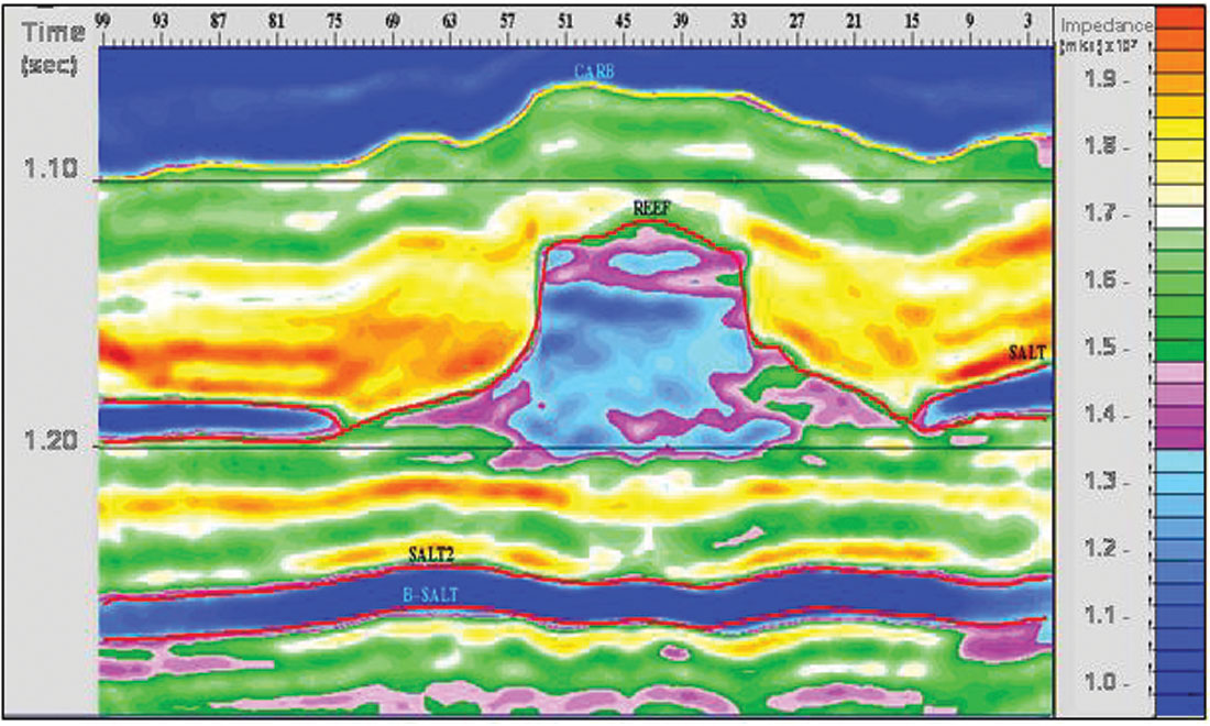
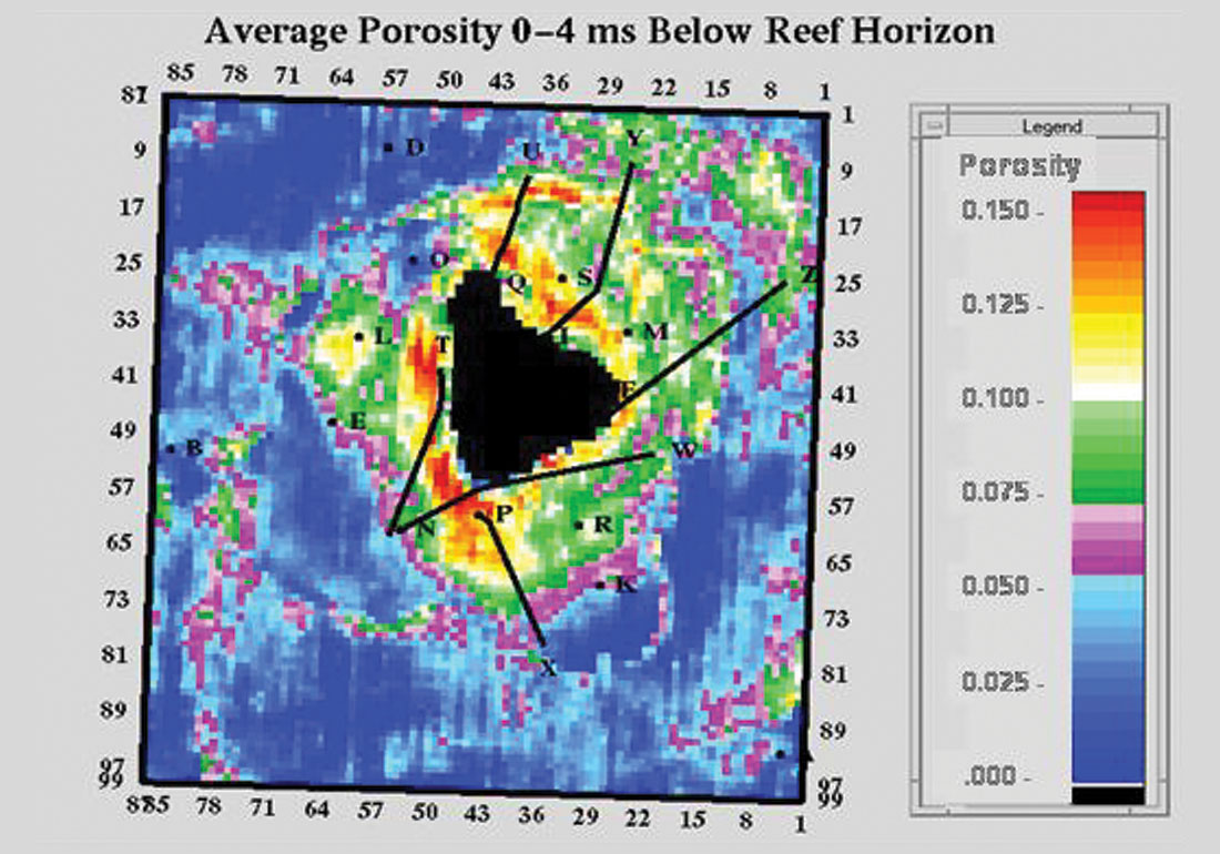
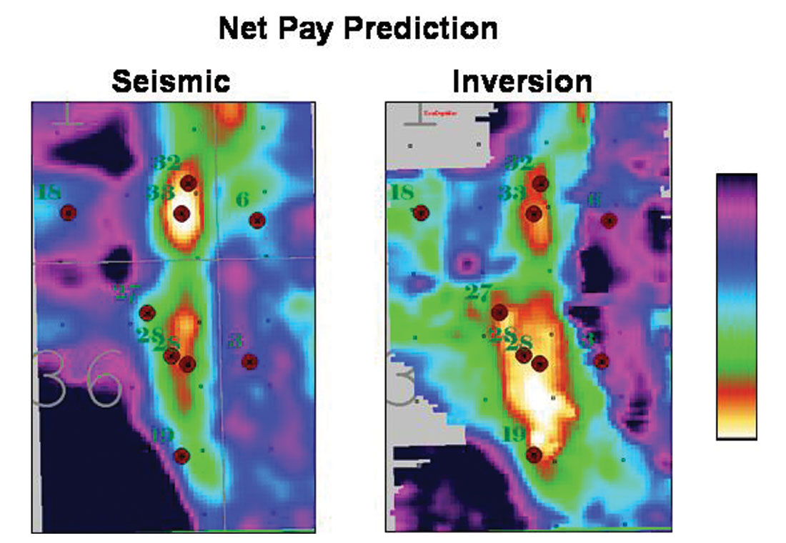
An example of the mixed-norm approach is shown in Figure 1 from Pendrel and Van Riel, 1997. It is the post-stack inversion of seismic over a Western Canadian Devonian reef. The magenta colours represent the porosity of interest in the reef apron. Salt can be seen both beneath and dissolving up against the reef (dark blue) while high-impedance anhydrites (reds) onlap against the reef build-up. The P Impedance from inversion has been converted to porosity and mapped in Figure 2. Note the enhanced porosity to the northeast (windward direction) due to rubble falling from the reef. Figure 3 is an interesting example from Western, Saskatchewan (Caulfield et al., 2004) which compares the estimation of net pay from seismic and a mixed-norm inversion. Imaging of the channel sandstones was estimated to be twice as accurate from the inversion.

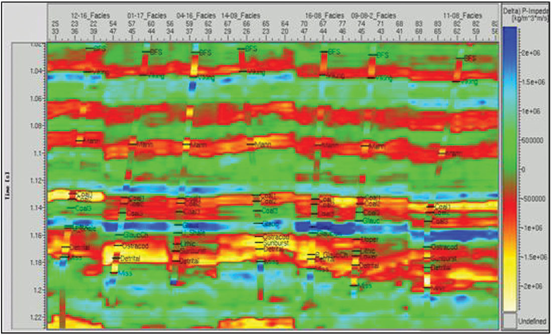
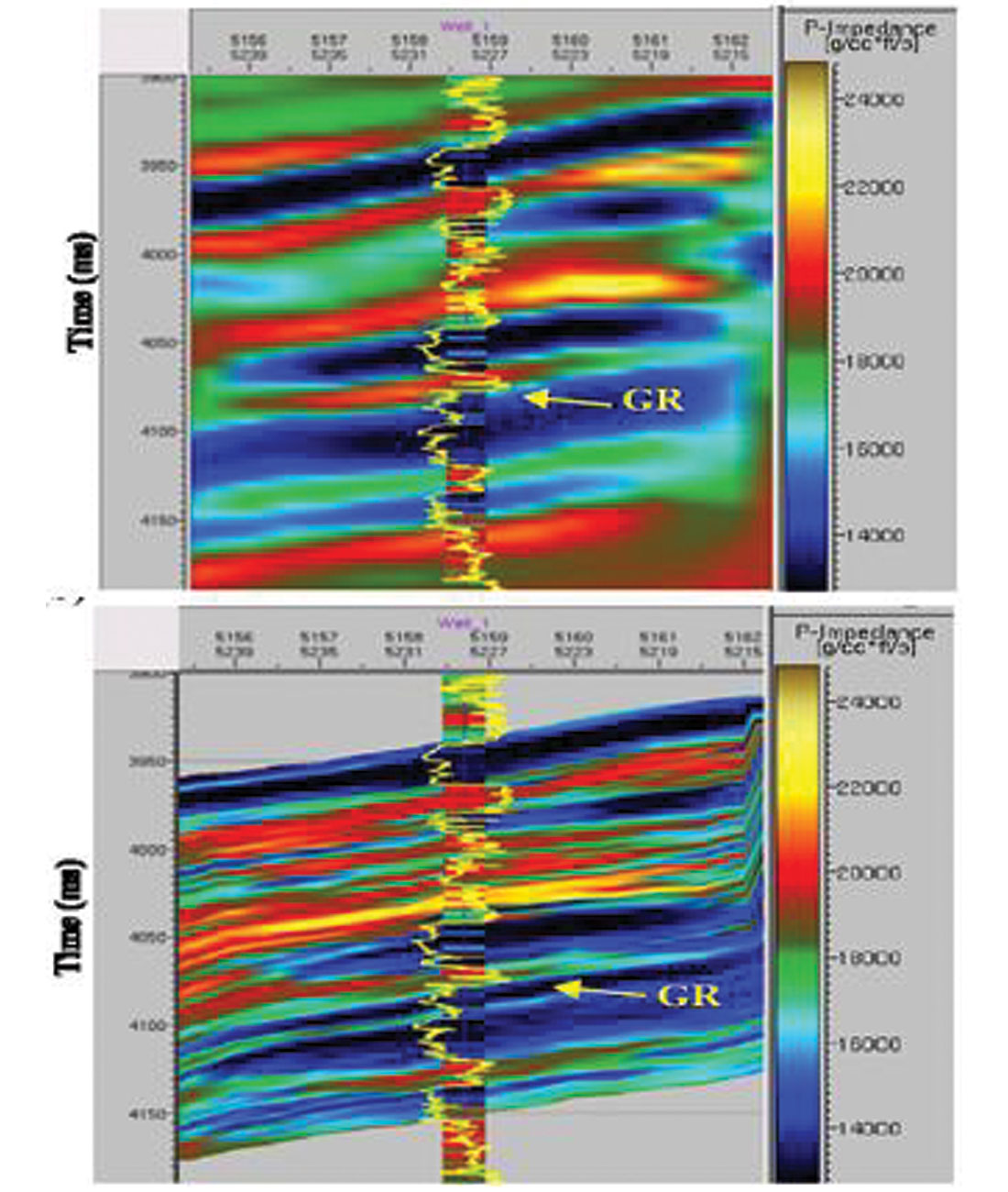
There always needs to be a good understanding of the contribution of the model frequencies to the seismic inversion. Their primary use should be to add low frequencies and thereby provide a geologic context in which to place the inverted seismic data. When they are used to add high frequency information in or above the seismic band, great care should be exercised. The model contribution can be constrained in a variety of ways, both inside and outside of the objective function. For example, it can be implemented either as a hard or a soft constraint. In any event, we need to very clearly isolate the unique and separate contributions of the seismic and the model. We can speak of two distinct inversion products. The relative inversion contains no low frequencies - it is the seismic data speaking to us directly. The absolute inversion on the other hand, does contain low frequencies from a model or stacking velocities and can be used to estimate absolute reservoir parameters. Quality control of the relative inversion is easy when model information has not been directly used within the seismic band. Since the inversion procedure in this case is effectively blind to the logs in the seismic band, the inversion is free to disagree with the logs. It then follows that comparing the relative inversion and the band-limited impedance logs is a very powerful quality control tool. Figure 4 is such an example of quality control of a relative inversion with band-pass-filtered impedance logs. The agreement is certainly not perfect. Is the issue with the seismic or the logs (or both?).

Development of the various algorithms continued as attempts were made to improve resolution, attenuate noise and incorporate more information. Rules-based methods added individual reflection coefficients to the solution one at a time in an optimal way. Global inversion was introduced to incorporate many traces within the objective function at one time. The resulting simultaneous solution was a good noise attenuator. Other methods added new terms to the objective function to softly constrain lateral continuity (soft spatial constraints). Stratigraphy was also accounted for by some algorithms. Commonly, it was invoked within the low frequency model. Less commonly, it was imprinted in the seismic band component. This led to more non-uniqueness in the resulting solution space which was subsequently addressed by the so-called stochastic (not to be confused with geostatistical!) solutions such as simulated annealing.

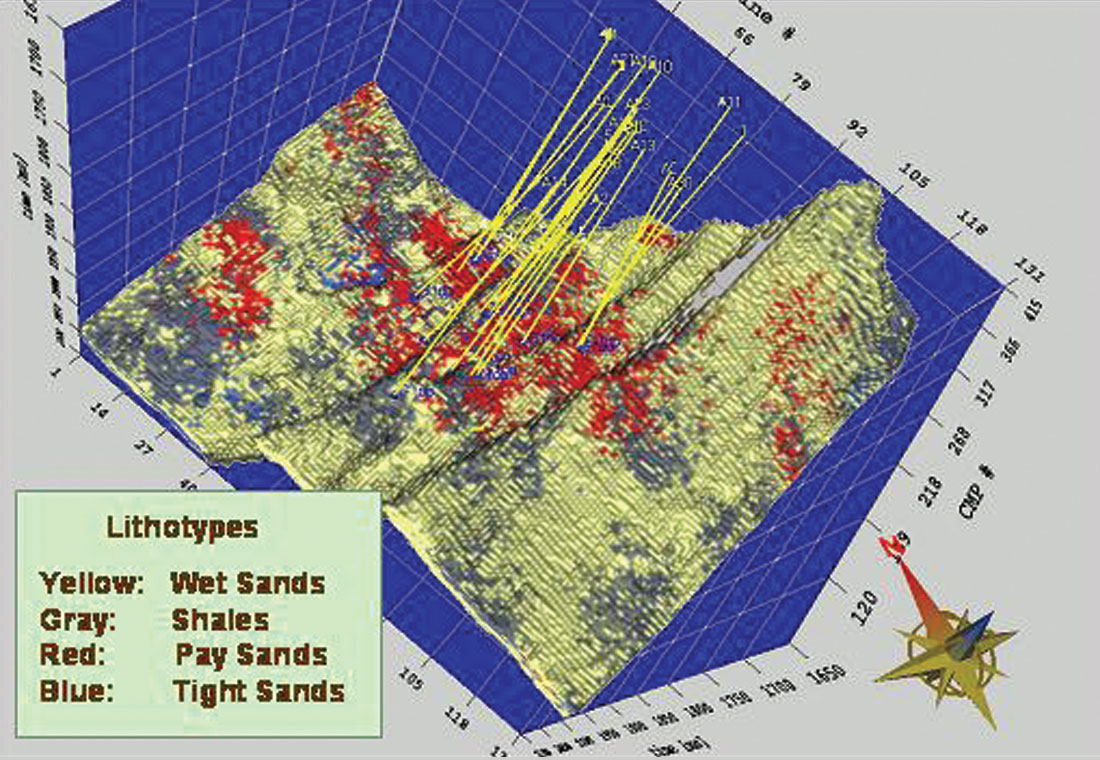
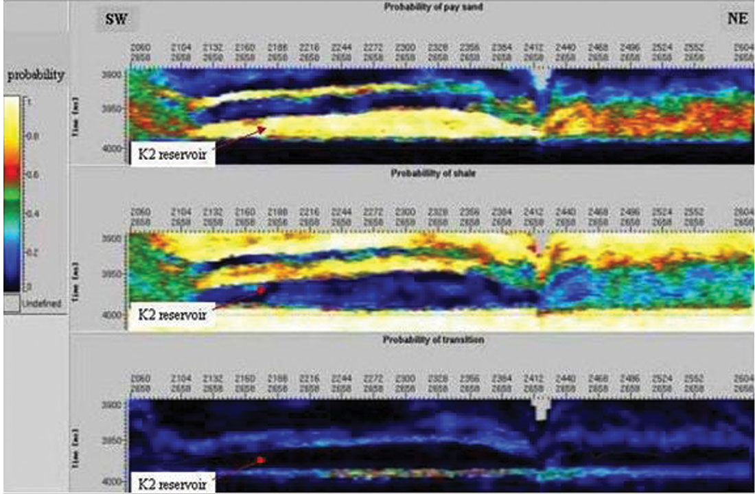
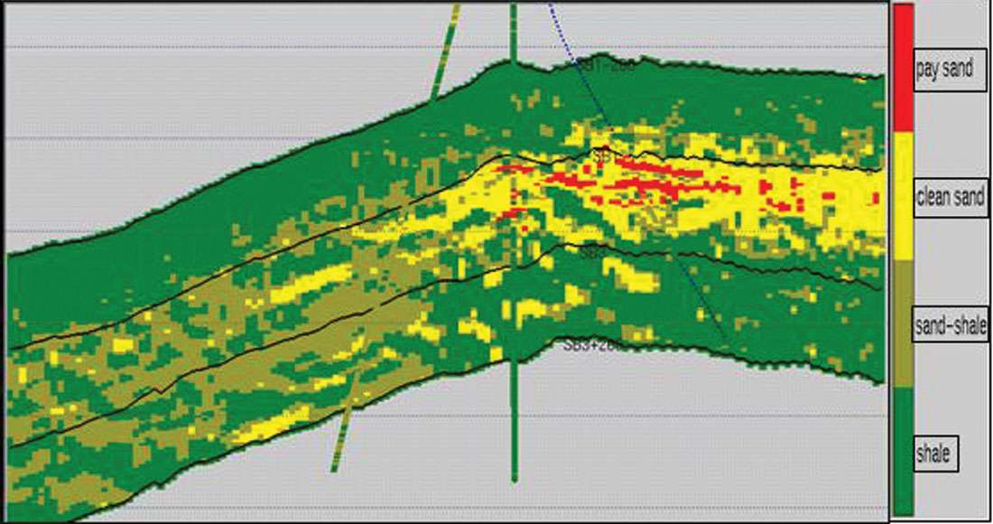
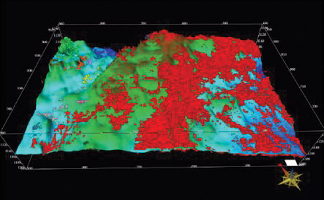
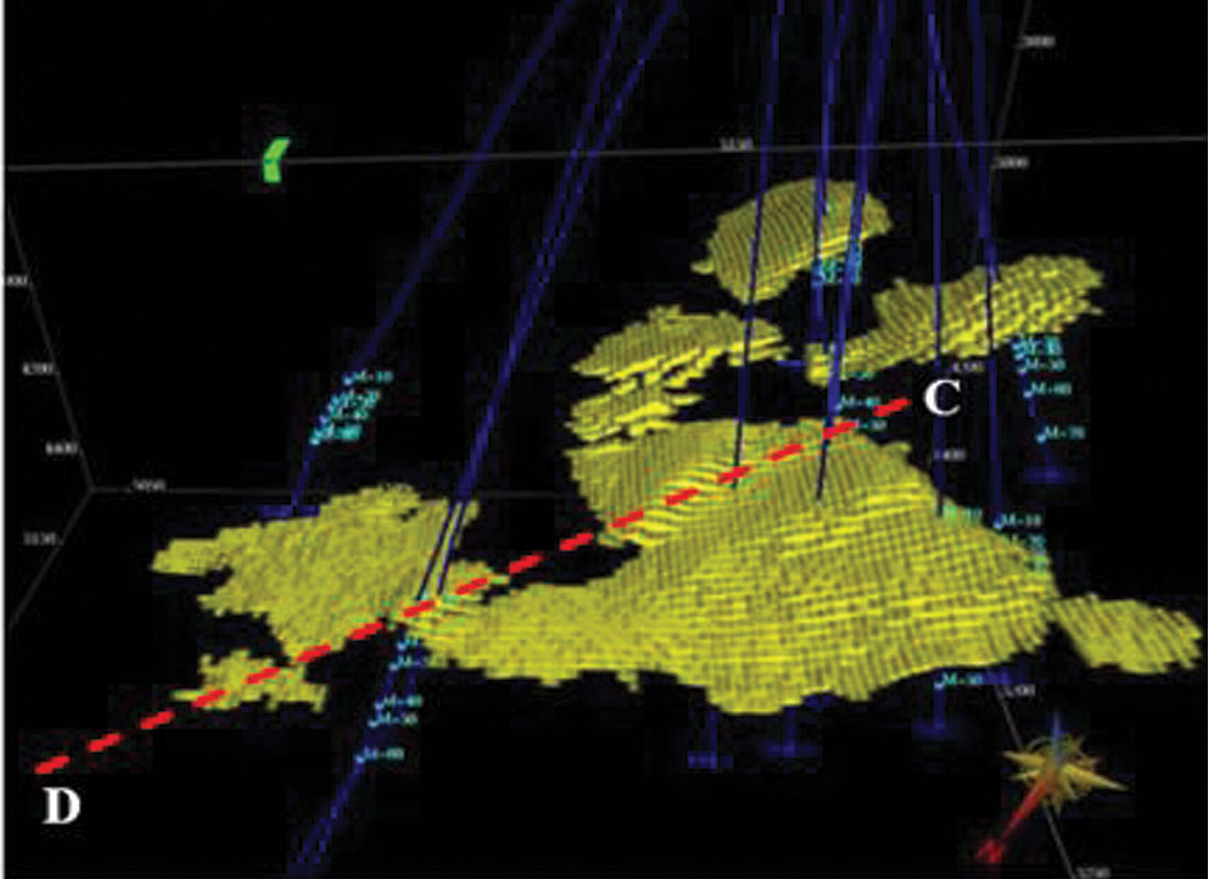
Non-uniqueness was always an issue, regardless of the algorithm used. This is a consequence of the band-limited nature of our data. Geostatistics provided a formal way of addressing this. Geostatistical Inversion formally merged these ideas and created the possibility of higher resolution along with formal estimates of uncertainty (Debeye et al., 1996). It ensured that all geostatistical realizations were consistent with the input seismic data. Latimer et al., (2000) combined Sequential Gaussian and Indicator Simulations with Geostatistical Inversion to determine the possible distribution of pay sands in the Gulf of Mexico. Figure 5 is an example of one realization from the set created. In Figure 6, the pay sands have been isolated and interpreted by an automatic procedure. Logs were used as a priori information in these approaches, leading to uncertainty estimates which were spatially dependent – increasing as distance from wells increased. A proper accounting for the distribution of the values within the set of realizations can lead to formal estimates of uncertainty and probability. Sullivan et al. (2004) applied these ideas to determining the probability of the location of sandstones within a three- facies depositional sequence (Figure 7).

We also saw the first attempts at implementing AVO inversion. Smith & Gidlow, 1987 showed how weighted stacking of NMO gathers could be used to estimate P and S reflectivity. While the term reflectivity is commonly attached to this method, it is a confusing nomenclature, since the wavelet remains within the data. An inversion of each reflectivity is required to remove it. A further rationalization ensures that the shear estimates are within reasonable bounds. Another limitation is the implication of a common wavelet for all offsets with no frequency loss at the far offsets.

Important work in AVO analysis was done by Goodway et al., 1997 who recognized that facies and fluids were often best-discriminated on cross-plots of the modified Lame’ parameters, LambdaRho (lambda*density) and MuRho (mu*density). This LMR technique has found application in both clastic and carbonate regimes.

The Modern Era – From Inversion to Facies

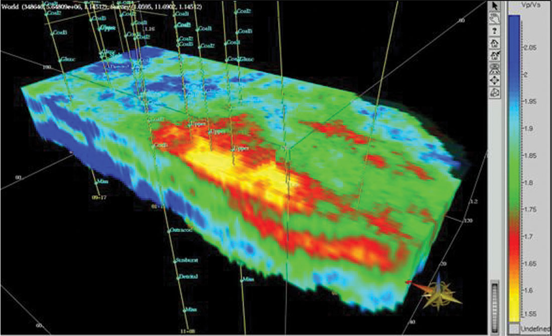
AVO inversion came of age with the implementation of the Simultaneous technology (Pendrel, Debeye et al., 2000). Simply, this means that partial offset or angle stacks along with their individual associated wavelets are input to a single procedure which computes P Impedance, S Impedance and Density at once. Density is not well constrained unless angles in excess of about 55 deg are available. In addition, analysis of and compensation for anisotropy must be made as the latter has an equal contribution to the AVO effect. The lowest frequencies are still specified from models – although now three are required. Various strategies for noise modelling and attenuation are available within the algorithms and different parameterizations are available (e.g. S Impedance, Vp/Vs). It has also been recognized that NMO correction to subsample accuracy is necessary for reliable shear estimates – not an easy task when the correct alignment is often visually mis-aligned due to tuning and possibly the AVO effect itself! Nevertheless, examples of the discrimination of sandstones from shales, impossible with P Impedance alone, have been spectacular. Less well known have been many carbonate successes – usually through the union of the Simultaneous AVO and LMR technologies. Figure 8 is a clastic example from Pendrel et al., 2000 which shows Vp/Vs from AVO Inversion for the Blackfoot Glauconitic sandstone. Fowler et al., (2000) used Simultaneous AVO Inversion to P and S Impedance to isolate hydrocarbon-bearing sandstones in the Gulf of Mexico (Figure 9). Guided by cross-plots of P and S Impedance from log data, the AVO Inversion was re-formatted in terms of facies as shown in Figure 10.

An immediate consequence of the idea of simultaneous inversions was the possibility of Joint inversions consisting of multiple modes – PP, PS, etc. Alignment and bandwidth issues are even more daunting here but not without solutions. In particular, PPPS holds the promise of direct detection of density at lower angles, without any type of Gardner or other assumption or constraint.

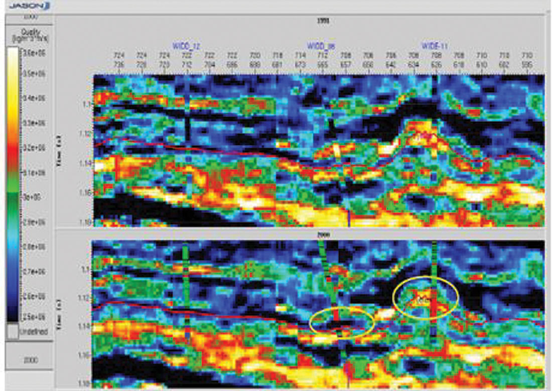
AVO and Joint Inversion also have application to 4D. The potential wavelet differences between vintages are easily handled by inversion. When the low frequency component is understood to be unchanging through time, a Joint PP-PP inversion of all vintages is useful in creating a high single baseline. Then, separate inversions of each vintage, using low frequency models derived from the baseline, can be done to extract 4D reservoir properties. Figure 11 shows a Southeast Asia example from Mesdag et al., 2003. In the Figure, AVO Inversion has been applied to the older vintage to identify hydrocarbon-bearing sandstones. AVO inversions were then completed on both vintages and reservoir measures were computed. In this case, the measure was the distance above the shale line on a cross-plot of S Impedance vs P Impedance. Log cross-plots showed that the difference of the measures between vintages could be used to determine changes in fluids. Figure 12 compares the measures from the two vintages. Regions where water has replaced oil are indicated.

Rarely are explorationists interested in rock properties like P Impedance and Vp/Vs directly. More importantly, they need to know about facies distributions, the volume and types of shales, sandstone quality and hydrocarbon content. Engineers care about porosity and permeability. We usually become forced to talk about impedances and densities as they are things that can be directly measured by the seismic reflection method. The comment “now I have an inversion, what do I do with it?” has been heard by the author on more than one occasion. Happily, all inversions can now be translated to facies/fluids domain (Pendrel et al., 2006), complete with their probabilities of occurrence at each voxel. Seismic attributes or even airborne e/m measurements can be combined with inversions for enhanced definition of reservoir property distributions.

Facies can also be estimated directly through the unique combinations of Geostatistical Inversion with Sequential Indicator simulation. The Geostatistical methods offer high resolution with uncertainty (i.e. probability) estimates. In addition, many realizations or possibilities can be generated – all consistent with the input seismic and well data. These can be of great interest to reservoir engineers who wish to test different scenarios against production history information.

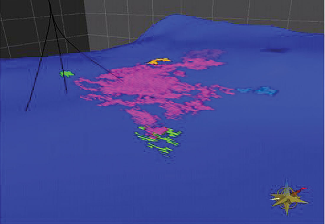
Throughout the development and evolution of inversion methods, there has been a continued interest in combining inversion techniques with other methods toward a better product. Typically, the techniques have been cascaded; inversion has been run followed by something else. The various methods have been difficult to assess because of the wide variety of inversion methods which have been used. Naturally, inversions which leave information "on the table" are going to benefit more from a follow-up procedure. Recently, disparate techniques have been united within a common inversion framework. Levering upon the often subtle patterns discernible from a multi-channel (i.e. multi CDP) analysis, effective resolution can be increased. The methods work for both post-stack and AVO and can incorporate well information formally or not. When incorporating well logs a priori, the methods can look very "Geostatistical" with multi-realization and probability estimates available. A clastics example from Contreras and Torres-Verdin, 2005 is shown in Figure 13. The upper panel is a traditional inversion. The lower panel shows the result from high-resolution Simultaneous AVO Inversion. In Figure 14 is a single sandstone body extracted from the mean of 10 high-resolution inversion realizations.

The Road Ahead

Looking back at the last five years, we have witnessed a startling integration of reservoir characterization processes. Disparate types of measurements such as airborne e/m and seismic can now be merged through inversion and facies discrimination. Geostatistics has been seen to be nothing more than a high resolution inversion with spatial uncertainty estimates where wells can be turned on or off to suit the convenience of the explorationists. Is it really still Geostatistics? Perhaps not exactly, in the classical sense. Semantics aside, it is of primary importance to use all relevant information toward estimating reservoir properties. So where do we go from here? It is interesting to note that our high resolution reservoir estimates are often de-sampled through a process known as up-scaling, before being used as input to a reservoir simulator. Together with production history data, they are inputs to a simulation process, which might take many days or even weeks to complete. We see ahead a continued integration process where high resolution reservoir property estimates can be used directly in fast simulation processes. The additional challenge is that they must run more quickly.

We also see a continued effort toward refining present reservoir property estimation techniques. AVO Inversion incorporates partial offset or angle stacks – sometimes as many as twelve. While AVO resolution would be best served by using NMO gathers directly, partial stacks have higher S/N and facilitate the sub-sample NMO corrections necessary for accurate results. However, with the aid of multi-channel pattern recognition techniques, inversion of individual NMO traces should be possible, while, at the same time, preserving the high accuracy in NMO which is required. There are further benefits. A full wave equation method should be able to better account for multiples - long a problem for seismic inversion algorithms. In principle the inversion and the wavelet estimation could be done simultaneously – and all this with proper accounting for multiples and peg-legs.

Since the author’s early days as a young researcher at a major geophysical research laboratory, it has been quite a ride! If the first generation began in the fifties with the likes of Robinson, Treitel and Wiggins, then we were the second generation. We were there for the development of wave equation migration, slant stacks, AVO and tomography and the beginning of the evolution of inversion. Now the third generation has arrived. They are in our university graduate programmes and, I believe, already in the offices of oil and gas companies right now. They will lead us to an exciting future – one which this author is eagerly anticipating.