Introduction
It is fair to say that surface seismic data are the staple of the typical oilfield geophysicist’s diet and that gamma ray and porosity logs provide the nutrients required by petrophysicists and geologists. The acoustic, or sonic, log, however, is the ketchup (or condiment of choice) used liberally by both parties, although often for different purposes. The sonic log brings together familiarity, biases, and expertise from geophysics, geology, petrophysics, and geomechanics. For example, the borehole scale and environment and details of logging are most familiar to the typical petrophysicist, but the waveform components important in modern sonic logging are typically a domain of expertise of the geophysicist. The sonic log is, then, a point of mutual comprehension and it is important that geophysicists understand what they are getting and what is behind the sonic log. This article aims to provide an introduction to the history of sonic logging, its evolution, and the basic principles of operation for the various flavors of sonic tools available today in the oil field.
A Brief History of Sonic Logging
Although a clear line exists between today’s sonic logging and borehole seismic surveying, both methods are organic continuations of the surface seismic techniques employed since the 1920s in oil and gas exploration. An obvious interpretation problem for pioneering seismic interpretation geophysicists was the correlation between time and depth. Although the speed of sound was well known in a variety of rock types, predicting the exact depth to any given reflector was not possible in all but the simplest of geological environments. In 1927 the recently incorporated Geophysical Research Company, a subsidiary of Amerada formed by the legendary Everette De Golyer, began making velocity surveys by setting off explosions on the surface and recording arrival times at known depths within a wellbore, thus providing some details of the time-depth relationship at the wellbore.
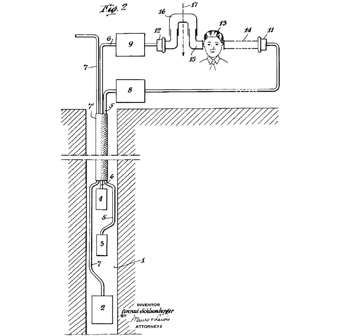
By 1935 Schlumberger Well Surveys Inc. began to offer its wireline truck and cable as a commercial service to seismic companies for wellbore velocity surveys. The fundamentals of acquiring checkshot data on wireline cable have not changed substantially since the technique’s inception. What has changed, however, is the cost. Inflationary pressures have driven the price upward from the $50 for five hours of surveying in 1935 (Edmundson 1985, Schlumberger internal document). Coincidentally, in 1935 Conrad Schlumberger was issued the first patent on what would now be considered sonic logging. It specified how to use a transmitter and two receivers to measure the speed of sound in a short interval of rock traversed in a wellbore (Schlumberger 1935). Figure 1 illustrates the proposed method, which failed at the time because neither logging engineers (unsurprisingly perhaps) nor the technology of the 1930s could detect the very short time difference between signals arriving at the two receivers.
The method proposed by Schlumberger differed from other methods of the day: It would provide a local measurement of even a thin layer, which could not be achieved by any other technique in use at the time. To this day, this describes the fundamental difference between the checkshot, or velocity, surveys that provide the broad changes in velocity with depth and the sonic logs that provide fine-scale refinements of the time-depth relationship given by a checkshot.
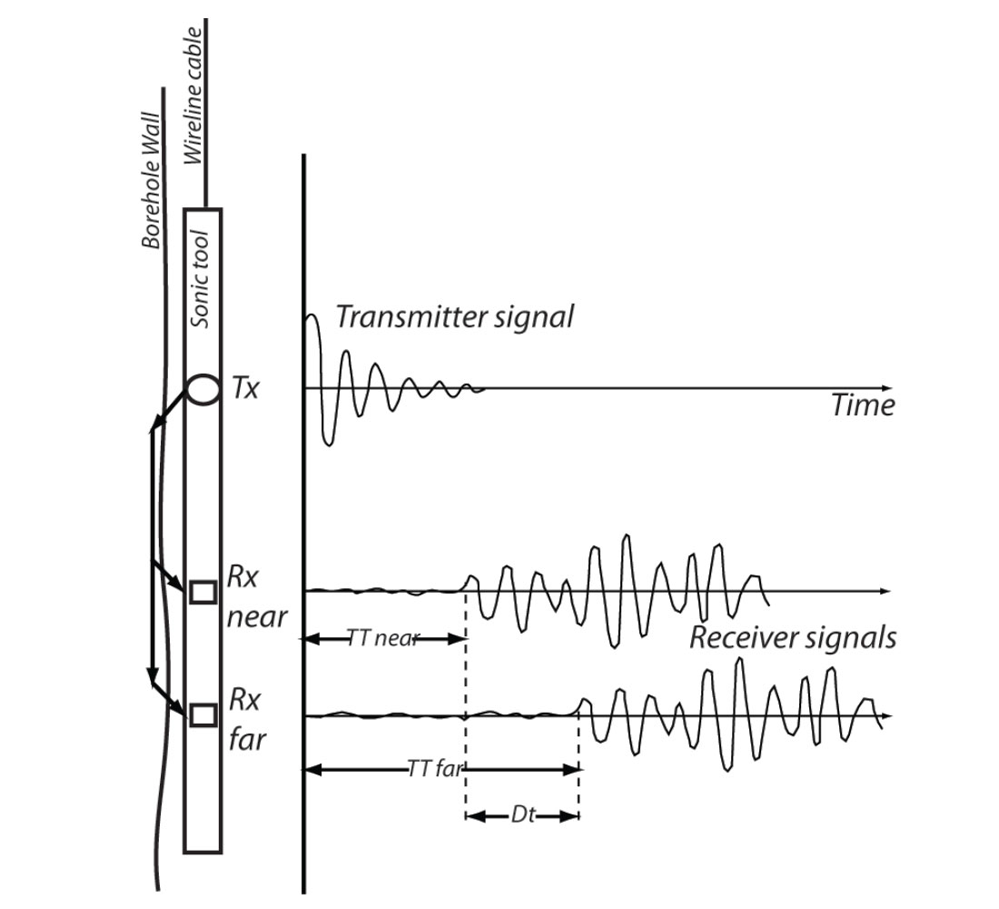
At least three oil companies independently built on these ideas in attempts to measure local formation velocities; more detail than available from well velocity surveys was needed to correlate observed reflections to lithological sections. Of the companies —Magnolia (later Mobil), Humble (later Esso), and Shell— Humble was the first, in 1951, to announce and build a continuous velocity logging tool (Edmundson 1985, Schlumberger internal document). The principle of the technique, measuring the difference in transit times using a single transmitter and two receivers, is illustrated in Figure 2. This transit time difference, or delta time (Dt or Δt), is defined as the slowness and is typically reported as time per unit distance (generally μs/ft or μs/m); it is, by definition, the inverse of velocity. The principle of today’s sonic technique remains very similar, over 50 years later.
The only known application of this new sonic logging tool was in the improvement of seismic data interpretation. However, this was soon to change. During the early 1950s Gulf Oil Corporation researchers were conducting acoustic experiments on real and synthetic porous media. The names of some of these researchers, such as Wyllie and Gardner, remain familiar to geoscientists today because of laws bearing their names. Their results included the time-average formula, which correlates sonic travel time and porosity (see Equation 1). These experimental results created a whole new avenue of opportunity for sonic tools and in a large part fulfilled the vision of Conrad Schlumberger’s 1935 patent.

Nuclear logging has now largely supplanted sonic logging for porosity determination, although the sonic porosity reflects primary porosity and not total porosity. Thus, the difference between the two can be a useful indicator of secondary porosity, and both compressional and shear sonic data can be used as gas indicators.
Additionally, sonic logs are still used widely as originally intended, to improve the correlation of time and depth, and are commonly used in rock mechanics and cement quality evaluation. Ultrasonic methods have also been developed for evaluation of casing and high-resolution analysis of cement quality.
Waveforms in the Borehold and First Motion Detection
Compressional (P) and shear (S) body waves are familiar to geophysicists who work with surface seismic data. Sonic waves in the borehole are simply higher-frequency and shorter-wavelength versions of these waves. For example, a typical 10 kHz sonic wave propagating in a 5,000 m/s formation has a wavelength of 0.5 m, in contrast to the wavelengths that measure in the tens of meters in surface seismic surveying. The wavelength and receiver geometry control the vertical resolution of the sonic measurement, typically estimated to be a quarter of a wavelength (Kallweit and Wood 1982). In the borehole environment, however, components other than body waves are also significant.
The compressional wave generated by a transmitter converts to refracted compressional and shear waves after it meets the borehole wall. The critically refracted wave components create head waves that transmit the formation body waves to the transmitter. However, if the formation shear slowness is greater than the borehole fluid slowness (i.e., fluid velocity greater than formation shear velocity), which is relatively common in slow formations, no shear component can be critically refracted along the borehole-formation interface. Hence, the shear wave propagating in the formation cannot create a head wave and therefore cannot be detected by the tool. Predicted by the laws of reflection and refraction defined by Willebrord Snellius (Snell’s law), this limitation has largely been overcome with advanced transmitter technology, but more about that later.
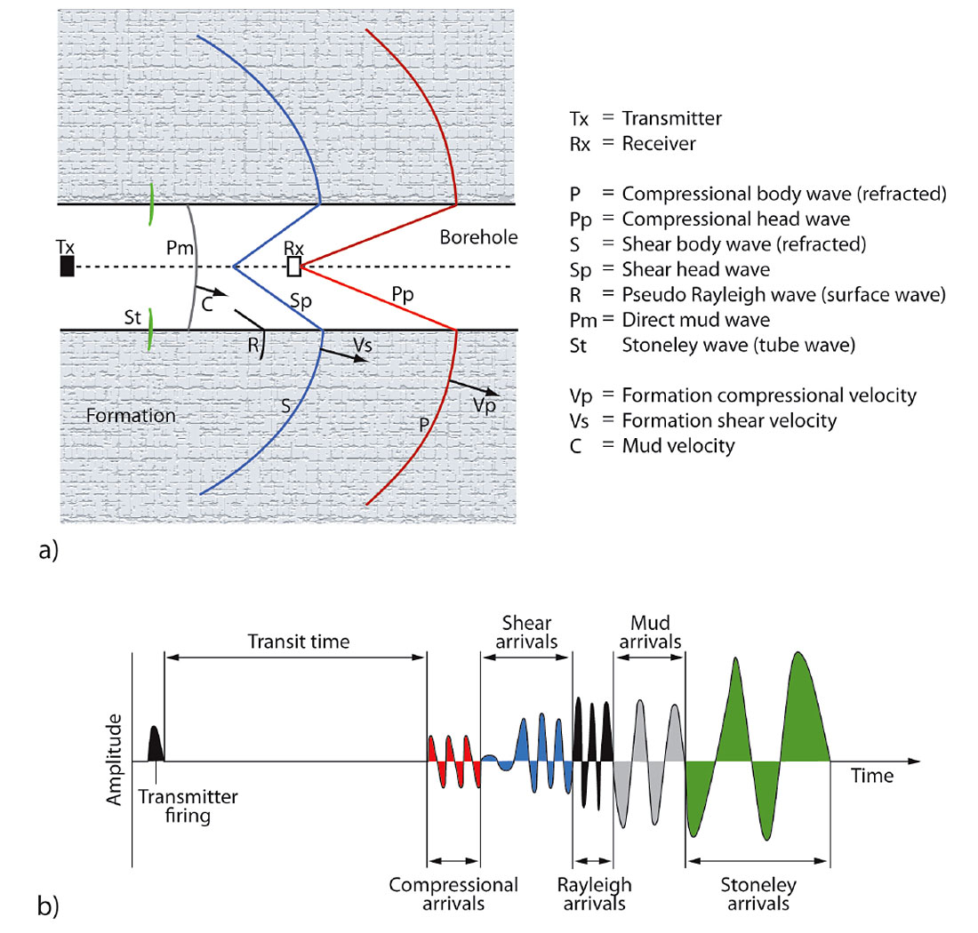
The important wave components generated by the transmitter in a formation where formation shear wave velocities are greater than the borehole fluid velocity (i.e., head waves can be created by the formation shear wave) are illustrated in Figure 3. In chronological order, following the arrival of the P and S head waves, are the following waves (after Brie 2001, Schlumberger unpublished report):
- Pseudo Rayleigh: a surface wave transmitted at the formationfluid interface characterized by elliptical particle motion. The wave is essentially controlled by the shear velocity of the formation, but is slightly slower. In most instances it is mixed with the shear arrivals in the waveform.
- Mud: the next arrival, theoretically, should be the compressional wave transmitted by the borehole fluid. However, the borehole is usually too small with respect to the wavelength and the transmitter-receiver spacing, and the mud wave is rarely present in a borehole.
- Stoneley: another surface wave with elliptical particle motion. This wave is always slower than the direct mud wave and has a large amplitude since the energy is guided in the borehole. Unlike body waves and head waves (associated with P and S wave propagation), which are nondispersive in a homogenous isotropic medium, the Stoneley wave is a dispersive wave and the propagation velocity is a function of the individual Fourier components.
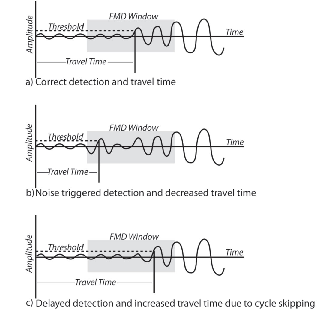
The received waveform clearly contains a large amount of information. However, the Dt measurement is based on detecting only the first or highest velocity energy transmitted by the tool transmitters, known as first-motion detection (FMD). Based on a number of parameters (rock type, borehole size, and fluid type) an engineer can predict the arrival time of the first energy for any given tool configuration to optimize the effectiveness of FMD.
The slowness values for typical formations encountered in the oilfield and for drilling mud types are included in Table 1. The engineer can set time-based gating parameters such that the software implementing the FMD is less likely to trigger on the borehole noise associated with tools and associated jewellery (centralizers, standoffs, etc.) being dragged through the wellbore. A threshold value also must be set, and it must be one that does now allow background noise that occurs within the detection window to trigger the FMD. The FMD process is illustrated in Figure 4.
| Material | Dt Comp. | Dt Shear | Dts /Dtc | ||
|---|---|---|---|---|---|
| μs/ft | μs/m | μs/ft | μs/m | ||
| Quartz sandstone (0 pu) | 51-56 | 167-184 | 88.0 | 289 | 1.59 |
| Limestone (0 pu) | 47.5 | 156 | 88.5 | 290 | 1.86 |
| Dolomite (0 pu) | 43.5 | 143 | 78.5 | 257 | 1.8 |
| Salt (halite) | 67 | 220 | 116.5 | 382 | 1.73 |
| Shale | >90 | >295 | variable | - | - |
| Coal | >120 | >394 | variable | - | - |
| Water-based mud | 200-210 | 620 | - | - | - |
| Oil-based mud | 205 | 672 | - | - | - |
| Casing | 57 | 187 | - | - | - |
| Table 1. A summary of approximate slowness values for various common materials in the oil field (Schlumberger Chart Book and unpublished material). | |||||
Noise is one of the major enemies of the FMD process; the other is cycle-skipping. Cycle-skipping occurs when the amplitude of the first arrival energy is attenuated such that it does not meet the threshold set by the engineer; the FMD skips this first arrival and is triggered on a subsequent and higher-amplitude part of the wavetrain. Cycle-skipping causes an increase in transit time and a falsely high Dt, whereas noise triggering causes a decrease in transit time and artificially low Dt (Figure 4). High gas saturation, unconsolidated formations, extreme washouts or caving, and gas-cut mud can all lead to amplitude decreases and therefore to cycle-skipping. However, even in ideal conditions the decrease in energy amplitude with distance from the source provides one of the practical limitations of offset available on sonic logging tools.
Sonic Logging Tools
By the late 1950s thousands of sonic logs were being recorded around the world every year by tools based on the original Humble design (Figure 2). There were several persistent problems with these tools and the logs they recorded. In particular, data was adversely affected in shale formations prone to alteration (damaged formation) and by wellbore washouts and borehole irregularities. The former problem was particularly evident if the transmitter-receiver spacing was small. In this case measurements were representative of the damaged zone only (similar to short offsets in a refraction experiment that sample only the near surface). A solution to the latter problem was found by Shell researchers, who proposed a technique to eliminate adverse effects from borehole irregularities (Vogel, 1952). In an advancement of this technique, eventually known as the borehole compensation (BHC) technique, transmitters were placed above and below multiple receivers, causing variations in transit times associated with washouts in the wellbore or sonde (tool) tilt to cancel out when the difference in the travel times are considered. The BHC sonic log became an industry standard after its introduction in 1964 and is still used widely today.
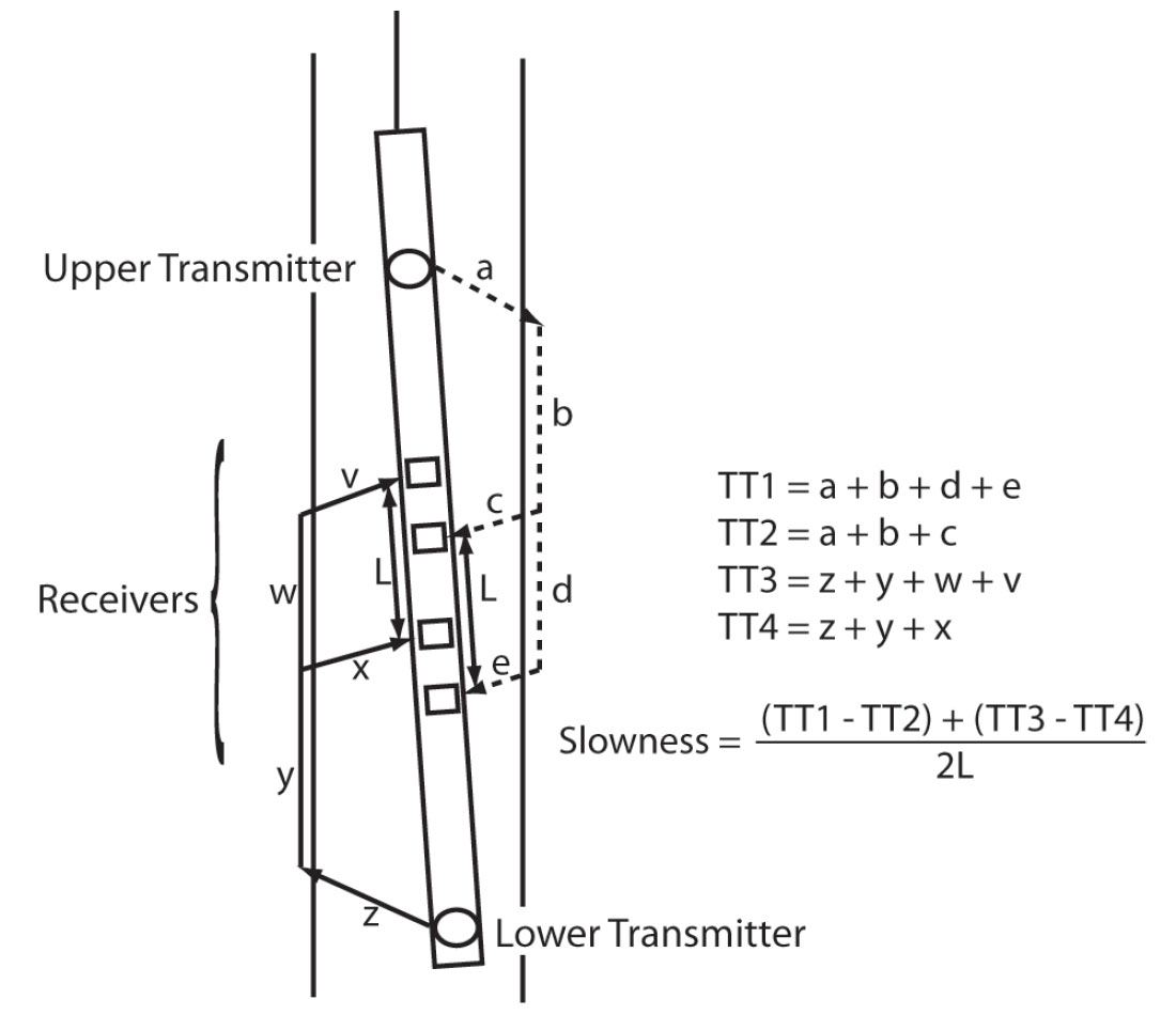
The fundamentals of almost all sonic logging tools are necessarily similar. At the most basic of levels, all sonic tools combine transmitters and receivers that allow the transit time of sound energy through the formation to be measured. The numbers and types of transmitters and receivers and their orientations vary depending on the complexity and the intent of the tool, but we will base this discussion on a standard BHC sonic logging tool comprising two transmitters and four receivers. The typical transmitter-receiver pairs (that is, with 3- and 5-ft spacings) and the simplified sound energy paths through the borehole fluid and formation are depicted in Figure 5. From these transit times the Dt can be easily computed as illustrated.
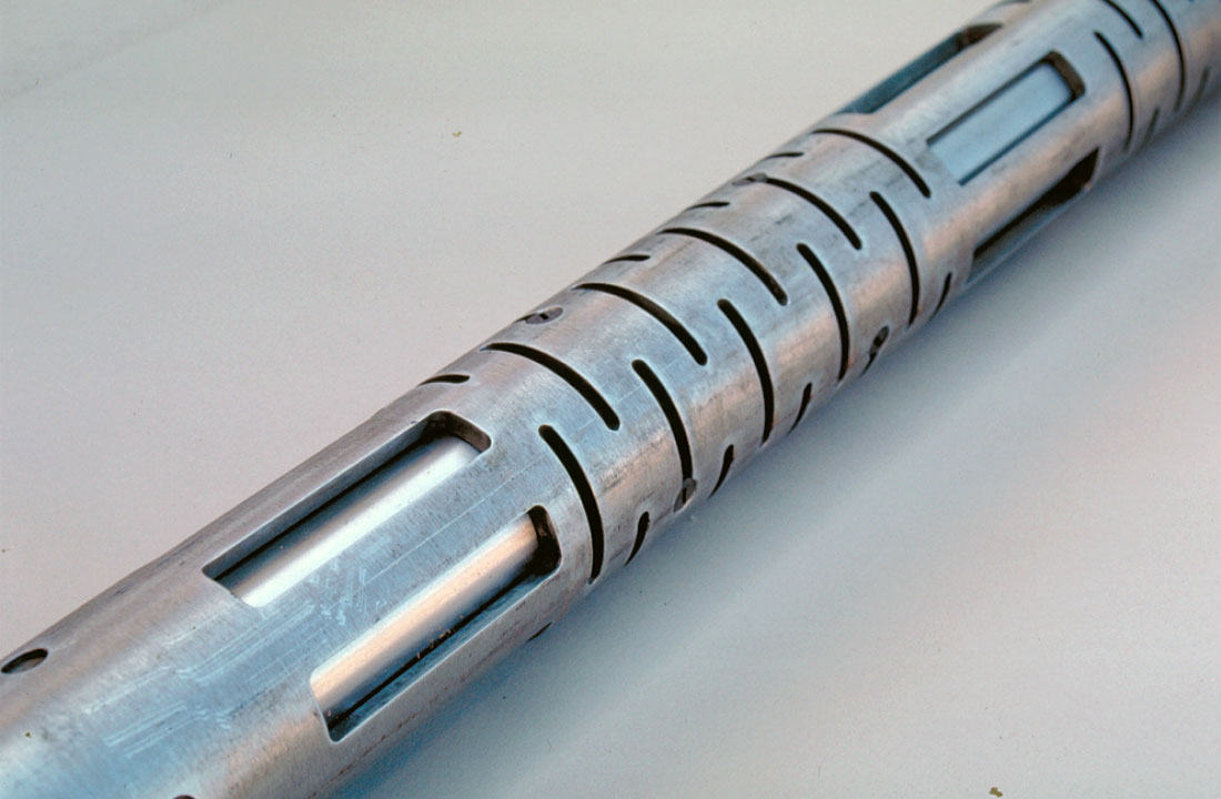
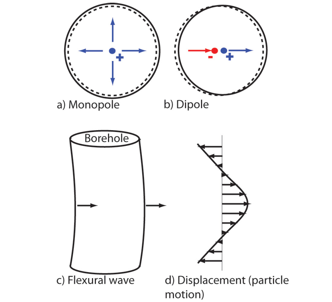
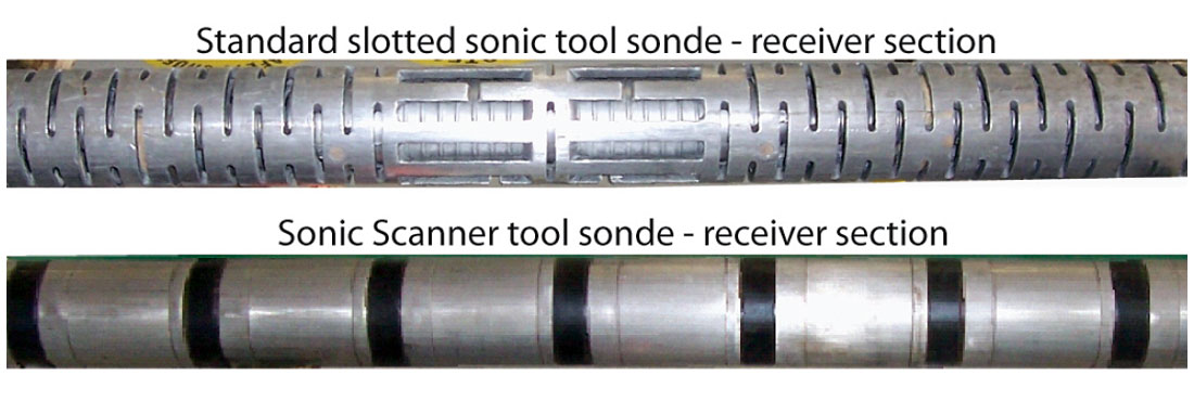
Transmitters in most BHC sonic tools are cylinders made of piezoelectric or magnetostrictive materials. An electric current is applied to the transmitter, which changes volume and generates a pressure wave or pulse that is transmitted in all directions. Physically, this source approximates a point source, or a pole, and is hence often referred to as a monopole transmitter. Receivers, usually made of piezoelectric ceramic, generate an electric current corresponding to the pressure variations in the borehole fluid around the tool. The frequency range of a typical sonic tool is 5 to 15 kHz, and the signal is therefore in the audible range of humans (~20 to 20,000 Hz). The click of a sonic tool can be heard from tens of feet when transmitting at surface. Most sonic logging tools are instantly recognizable by their characteristic slotted sonde or tool body that to the uninitiated vaguely resembles a spaghetti strainer (Figure 6). The slotted tool housing ensures that any direct arrivals of sonic energy transmitted by the tool body are slower than the signal transmitted via the formation.
In this way the BHC tool accounted for the effects of borehole irregularities and tools that were not centered within the wellbore. However, only the compressional wave energy was being consistently used and recorded using FMD, and further advancements in technology were required before other waveform components could be fully exploited.
Shear Wave Slowness Measurements and Dipole Sources
That recorded sonic energy contained information far above and beyond simply the transit time of the first energy arrival was understood well before it was routinely exploited. Shell researcher G.R. Pickett showed in 1963 that the time-average equation also describes shear wave velocity data and that the ratio of P-wave and S-wave velocities appeared to make a promising lithology indicator (Pickett 1963). However, recording the full waveform was not feasible with the computing and telemetry power of the 1960s. Oil and service companies alike worked on advancing sonic logging tools to allow full waveform recording and digitization. Engineering advances made increasing the number of receivers possible, and an important advance in signal processing, slowness-time-coherence (STC) (Kimball and Marzetta 1984), made receiver array processing for the various coherent waveforms robust. In 1985 the first array sonic tool was introduced that allowed downhole digitization of the full waveform possible (Morris et al., 1984). Delivering shear wave velocities was becoming a reality just as geophysicists were starting to better understand ”bright spots” and use amplitude variation with offset (AVO) analysis in the exploration workflow, which required shear wave data for model calibration.
Although important in AVO analysis, shear wave recording was still limited to zones of relatively fast formation. No advance in data processing can change the laws of reflection and refraction, so a fundamentally different technique was required to measure the shear wave slowness regardless of the slowness of the borehole fluid. The solution to this problem came in the guise of a new type of transmitter, a dipole transmitter.
Dipole transmitters are effectively pistons that create a pressure increase on one side of the borehole and a decrease on the other (plus and minus signs in Figure 7b), in contrast to the nondirectional monopole source (Figure 7a). Dipole sources are directional and focus their energy; in this way they contrast with standard or monopole transmitters that are omnidirectional, transmitting equally in all directions. Dipole transmitters excite a borehole wave mode known as a flexural wave, regardless of the formation shear slowness. The motion of a flexural wave along the borehole can be thought of as similar to the disturbance that travels up a tree when someone standing on the ground shakes the tree trunk. The analogy works even better if the tree trunk is fixed at the top and has a constant diameter (Haldorsen et al. 2006).
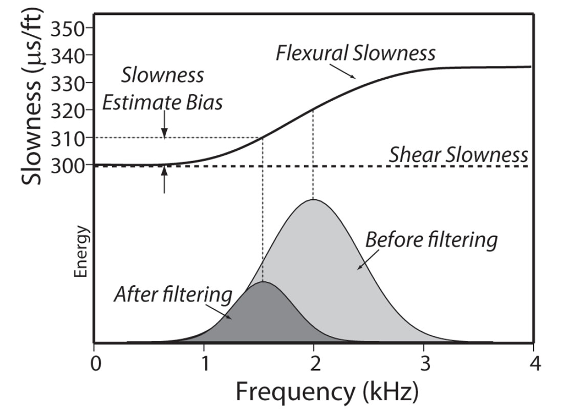
The utility of the flexural wave is that at very low frequencies its slowness equals that of the shear wave propagating in the formation. This implies that the flexural wave is dispersive, where different frequencies travel at different velocities. This makes dipole shear slowness determination more difficult and also introduces an error, or bias, in the slowness determination that must be corrected (Brie 2001, Schlumberger unpublished report). Typical slowness dispersion curves for the flexural wave are shown in Figure 8a, and it is clear that at low frequencies the shear and flexural waves have equal formation slowness values. Because it is difficult to excite flexural waves at these very low frequencies, a bias correction is generally required. By applying a low-pass filter to the recorded signal it is possible to enhance the signal of interest, reduce the effects of dispersion, and therefore the amount of correction or bias required (Figure 8b).
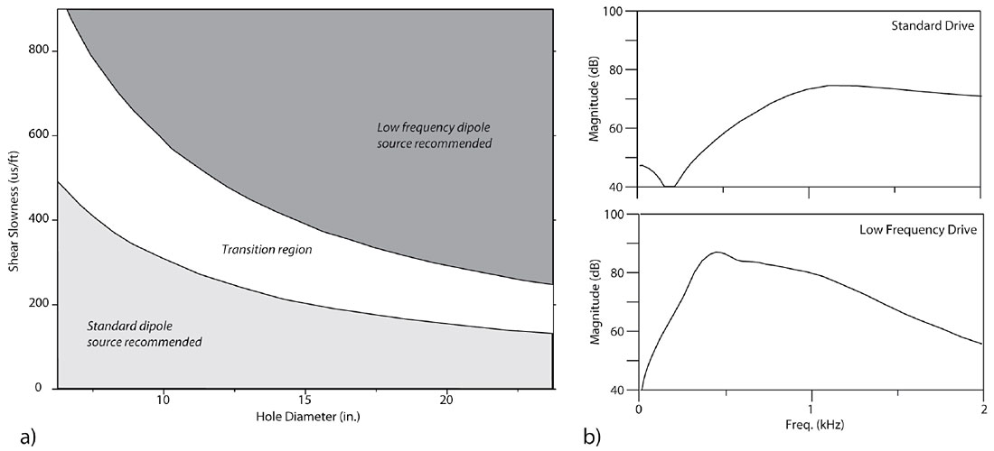
In addition to being influenced by formation slowness, the frequency content of the flexural wave is a function of borehole size. Faster formations and smaller boreholes typically require a higher dipole driving frequency for best results, whereas slower formations and larger boreholes generally require a lower driving frequency. The need to select an appropriate drive may result in two cases: Either multiple runs are required where there are major lithological changes or the borehole condition is very poor (i.e., diameter of the wellbore changes dramatically), or the wrong mode is selected if care is not taken in job preparation or if there is poor communication between the logging engineer and company geoscientists. The recommended transmitter mode for a range of slowness–borehole diameter values is illustrated in Figure 9, which also shows the amplitude spectra of typical lowand standard-frequency drives.
The combination of dipole sources, receiver arrays, downhole digitization, and improved telemetry allows recording of full waveforms, which include shear information in the guise of flexural waves. Obviously, FMD is not a useful method of analyzing these multiple arrivals. However, STC processing (Kimball and Marzetta, 1984) allows the different components to be identified and labeled to provide Dt measurements of individual components.
STC is a processing technique based on semblance analysis in a manner very similar to velocity analysis of surface seismic data. The STC process searches for coherent components in an array of waveforms recorded within a specified depth range in the wellbore (Figure 10a). Waveforms are analysed within a time window that for each time step through the recorded waveform analyses the semblance at a range of moveouts, which correlates to a range of formation slowness values. In other words, for infinitely fast formations the arrival time would be equal at all transmitter- receiver spacings and the moveout would be zero, and vice versa).
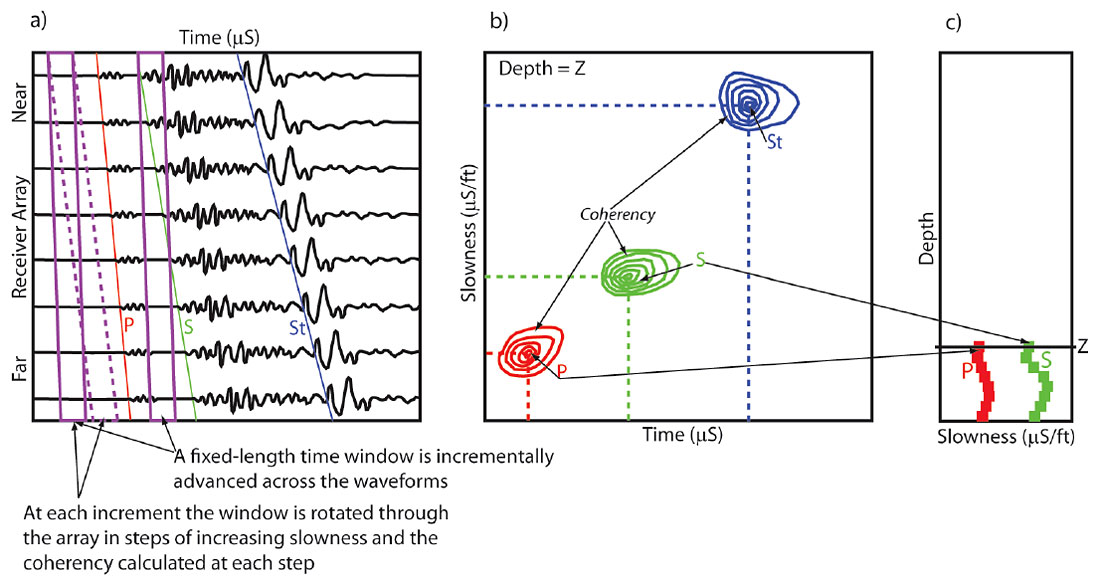
The typical method of analyzing STC results in log format involves two steps. First is the plotting of coherency or semblance as a function of time and slowness to create a slowness- time map for a given measurement depth (Figure 10b). Second is representing the coherence peaks from the time-slowness map as points on a log at that given depth. Repeating this process at all depths creates a continuous log (Figure 10c).
Since the 1980s STC processing and dipole transmitter technology have penetrated deeply into the wireline sonic market, although BHC logging for compressional Dt measurements remains common. Additionally, dipole sonic logging has grown to encompass a wide range of geomechanical applications, which have been important as long-reach wells and artificial stimulation of unconventional gas resources have become more common. However, the technology has remained largely unchanged since the 1980s and the sensitivity of the measurement has limited its applicability in some environments. In recent years a number of advanced dipole tools have reached the market. Their huge gains in better quality of data are responsible for new applications.
New Technologies and Applications of Sonic Logging
An important attribute of the dipole transmitter is that it is directional. This allows properties to be examined for anisotropy, which is very useful given that the half-space where most geophysics takes place is neither isotropic nor homogenous. When coupled with an inclinometry tool that can measure tool orientation, a sonic tool that comprises two sets of crossed dipoles (dipoles oriented orthogonally) can provide a measure of anisotropy in sonic and sonic-related properties. The sensitivity to anisotropy and quality of measurement are, predictably, dependent on tool design; more specifically, dependent on the types and designs of the transmitters, receivers, and sonde bodies.
By the 1990s, each of the major wireline service companies offered dipole sonic tools capable of measuring shear slowness and its anisotropy, if present. Until recently their respective technologies have been relatively similar. Most dipole sonic tools comprise, in addition to a standard monopole source, two pairs of orthogonal dipole transmitters, up to eight pairs of receivers (pairs are required to align with both dipole orientations), a slotted sonde body, and some kind of isolation joint between the transmitter and receiver tool sections. However, several important advances in technology were introduced with the Sonic Scanner (Mark of Schlumberger) tool in 2006 (Pistre et al., 2005).
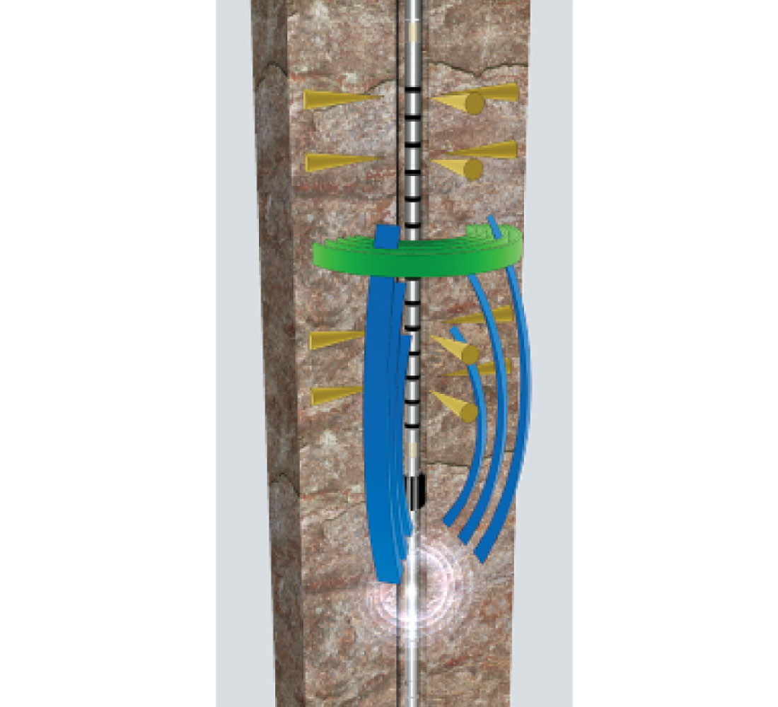
The design of the Sonic Scanner tool and many of its critical components are completely different to those of other sonic logging tools. The most obvious of these changes, at first glance, is the solid tool body without the slots characteristic of other sonic tools (Figure 11). The tool has been engineered such that the effects of its presence on sonic energy in the borehole can be modeled and accounted for. In previous tool designs, the effects of the slotted bodies cannot be effectively modeled and have unpredictable responses on sonic energy. This is not an issue for a basic Dt log, but for advanced processes or challenging conditions the tool itself is a limiting factor in the accuracy of its measurements.
The Sonic Scanner tool can provide full three-dimensional characterization of sonic propagation around the borehole. It is capable of acquiring axial, azimuthal, and radial measurements (Figure 12), each of which has utility in different environments and for different applications. This ability is partly a function of the fully characterized tool effects and partly because of a new type of transmitter and a vastly increased number of receivers.
The dipole transmitters, which are “shakers”, are designed to emit signal over as wide a frequency band as possible. This contrasts with other dipole tools, which maximize amplitude at the expense of a broad frequency range. A shaker comprises a suspended magnetic mass that is forced back and forth in a onedimensional plane by alternating electromagnetic forces. The shaker is contained within a shell that is itself also suspended within the tool. This configuration enables the shell to move in the opposite direction to the shaker and to generate a highfidelity dipole flexural wave in the borehole. One of the major benefits of this equilibrated action-reaction system is that, unlike dipole sources on previous-generation tools, the tool does not recoil in the opposite direction and create unwanted and uncontrolled interference.
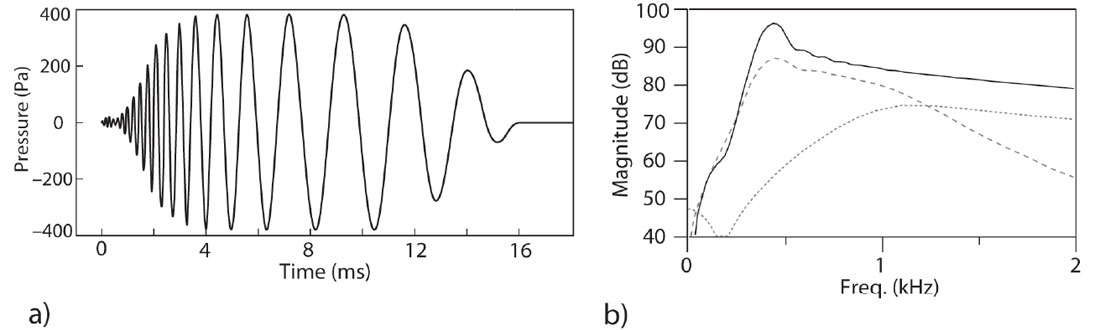
The broad frequency range, obtained by emitting a chirp-type signal (Figure 13), provides a number of benefits. Operationally, it is advantageous because the source signal is inherently optimized for all formation types and borehole sizes. This prevents the need for multiple runs with different frequency drives and removes the possibility of having a novice field engineer select an inappropriate frequency drive. The chirp signal outputs more energy than both the very low-frequency and standardfrequency drives of the dipole shear sonic imager (DSI (Mark of Schlumberger)) over the range of 0 Hz to 2 kHz (Figure 13).
A broadband signal is also advantageous as the large frequency content allows the dispersive waveforms to be analyzed quantitatively. Sonic dispersion analysis decomposes the recorded wavetrains into frequency and phase independent of arrival time.
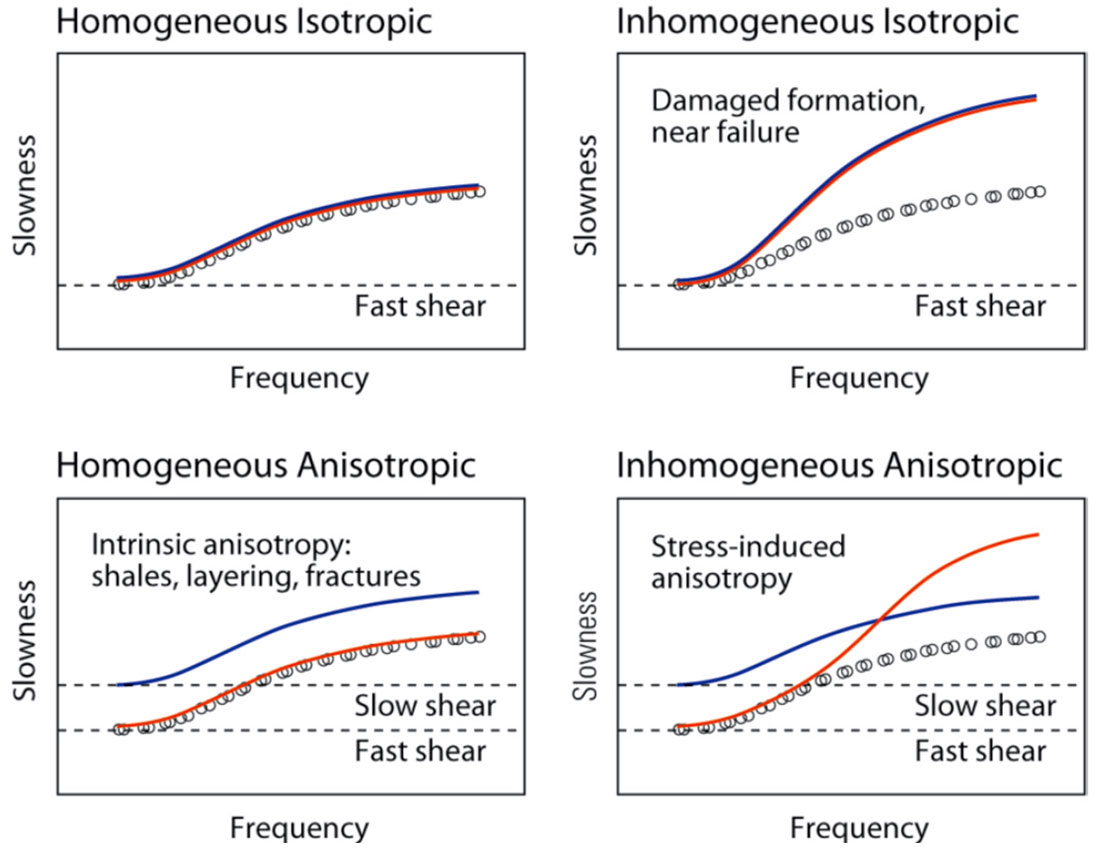
The dispersion of shear wave energy can be attributed to acoustic rock property variations that arise because of nonuniform stress distributions, mechanical or chemical near-wellbore alteration resulting from the drilling process, and intrinsic anisotropy related to the in situ properties of the formation. These property variations can be inferred from broadband sonic dispersion plots of propagating borehole acoustic modes. Figure 14 depicts several common scenarios with regard to fast and slow shear wave polarization, and it is clear from this figure that sonic dispersion analysis can identify not just the presence but also the type of anisotropy.
Recognizing the cause or causes of anisotropy is often very important. For example, the information is useful for recognizing the presence and orientation of natural fractures and determining the orientation of the maximum horizontal stress direction (which is critical to well planning if the formation requires hydraulic fracture stimulation to produce) and also, in geophysics, for understanding the effects of transversely isotropic media (Figure 15).
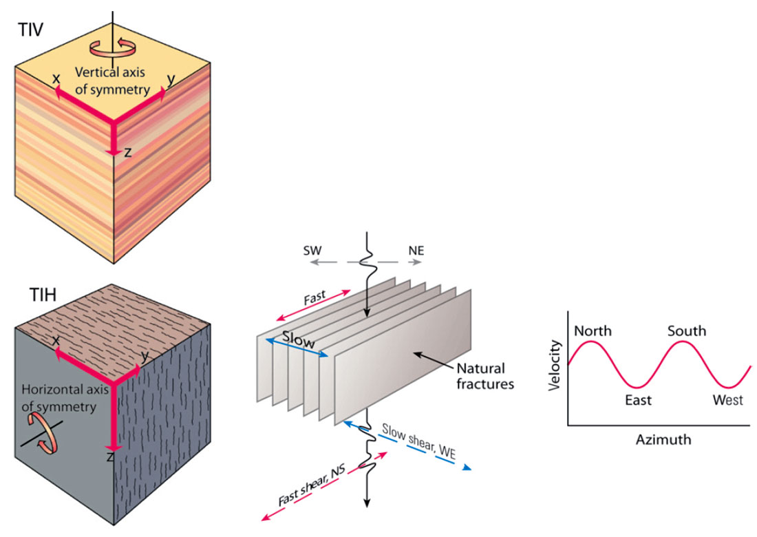
A vertically transverse isotropic (TIV in Figure 15) medium results in wave propagation velocities (compressional and shear) that differ depending on the direction of travel. Hence, if a well is deviated or if there are nonnegligible formations dips, the sonic measurements will be compromised because the measured values are a combination of the slow and fast vector components.
This is clearly not optimal where the vertical compressional and shear wave velocities are required, such as in AVO studies. The Sonic Scanner provides a means of quantifying and accounting for these effects by quantifying anisotropy.
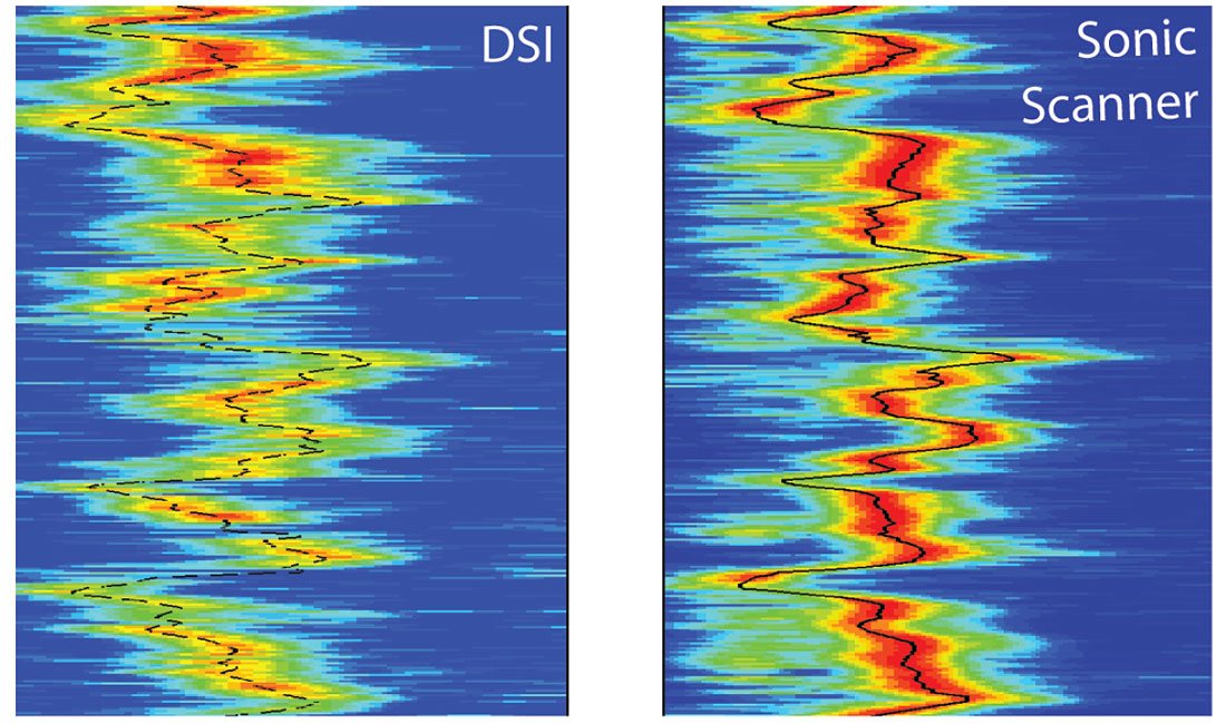
The tool engineering and characterization and transmitter technology contribute substantially to the advanced measurements and analyses that are possible. However, the receivers and monopole transmitters also deserve mention. There are a total of 104 receivers, and 13 receiver locations along the axis of the tool are each populated by eight azimuthal receivers. This leads to a far better signal/noise ratio and correspondingly improved STC coherency (Figure 16), and also to improved directional sensitivity.
One further technological advance of note is the configuration of the monopole transmitters. Although, the monopole transmitters themselves are not particularly unique, they are located such that near- and far-monopole measurements can be made. This allows radial profiling of the formation; the offsets possible with the far transmitter (11–17 ft) allow greater depths of investigation within the formation and therefore an increased likelihood of sampling virgin formation. This makes the tool the first in the industry that can measure and quantify the damage beyond the near-wellbore data available from formation imaging tools.
The radial profiling provides one means of quantifying the geomechanics of the wellbore and formation. However, the highquality three-dimensional measurements are also being heavily used as inputs for calculating rock properties such as Poisson’s ratio, Young’s modulus, and bulk and shear modulii. These formation properties control the physical behavior of the formation and assist in establishing the optimal mud-weight window and optimizing drilling and completion operations. But, the Sonic Scanner geomechanical application is a whole subject by itself and one that is outside the scope of this article.
Conclusions
The sonic measurement is one of the purest of log measurements. It requires very few assumptions and is largely unbiased by models relative to nuclear and induction tools. The concept of the technique has not changed profoundly since 1935, when Conrad Schlumberger penned the first patent for sonic logging as we know it today. However, advances in technology and our increased understanding of sonic waveforms in the borehole, largely through computer based modeling, have increased the applications of sonic logging far beyond those imagined in the early decades of exploration technology development in the 20th century.
Today, BHC and conventional dipole sonic logs provide most the sonic information required by petrophysicists, geologists, geophysicists, and geomechanics engineers. However, with the introduction of the Sonic Scanner technology and the increased quantity and quality of information now available, this is changing and will continue to do so.
There is much more that could be included in an article that seeks to explain sonic logging. It is simply not possible to include all the available worthwhile information without such an article becoming a book. We do hope, however, this article has some historical value, particularly for those readers who, like some of the authors, are a little too young to be intimate with the oil field’s unique history.

Acknowledgements
The authors recognize and thank the many colleagues who volunteered information and historical references for this article; they are too numerous to name individually here. Helpful reviews were also received from Dr. Peter Kaufman and an anonymous reviewer.
Related Reading


Join the Conversation
Interested in starting, or contributing to a conversation about an article or issue of the RECORDER? Join our CSEG LinkedIn Group.
Share This Article