Time-Lapse Survey Repeatability: An Elastic Modeling Study

Remote monitoring of fluid movement in a subsurface formation is an important application for seismic reflection imaging. In this setting, it is important that seismic data be acquired and processed in a repeatable fashion in order to reliably detect image differences due solely to the formation fluid changes. One way to explore the sensitivity of anomaly detection relative to seismic acquisition and processing is to create and process synthetic seismic data sets using numerical earth models representing different stages of fluid movement in a formation. For our study, we used a fast and efficient elastic modeling program to generate seismic surveys associated with ‘baseline’ and ‘monitor’ 2D earth models. Each monitor model differed from its corresponding baseline only in a small subsurface zone, where rock properties were altered to simulate formation fluid change. With identical acquisition and processing parameters for a baseline model and its matching monitor model, the detectability of an anomaly was surprisingly robust in the presence of both random and coherent noise. Even in the presence of significant simulated ‘seasonal’ near-surface variations, the test anomaly remained detectable. While we explored a number of models and acquisition scenarios in our original study, we summarize here by showing one significantly challenging example.

Introduction

Time-lapse surveys

The fidelity of seismic reflection imaging has improved significantly in recent decades, and in some cases, a modern seismic survey can reveal information about the fluids present in the pores of the rock layers. In such situations, it may even be possible to detect changes in the fluid content of the rock pores at different stages during production of an oilfield. More recently, stimulated by increasing concern about rising atmospheric CO2 concentration, various projects around the world have begun to study injection and sequestration of CO2 into porous formations, often in conjunction with tertiary recovery of hydrocarbon fluids from those same formations. In any case, it is useful to be able to remotely monitor the progress of fluid movement within a porous layer, in order to optimize engineering decisions. The most obvious approach is to design and execute a high-resolution seismic survey of the site before hydrocarbon production or CO2 injection begins, then to perform an identical survey after a specific time interval in order to compare with the baseline survey and detect the changes in rock properties due to the production or injection activities.

Obviously, it is important to repeat the seismic data acquisition and processing as carefully as possible, so that any changes in the results can be attributed to rock property changes, rather than changes in the acquisition parameters, or differences in the processing flow. As far as possible, repeated seismic surveys should be done using either the same permanently installed sensors, or at least common sensor positions. Also, if possible, repeatable sources like Vibroseis should be deployed, using common source points for all surveys. Even when the acquisition is duplicated as closely as possible, however, variations in the near surface properties due to seasonal changes (water table variations, frozen surface in winter) can affect the repeatability of seismic surveys.

Complexities in the earth itself affect seismic imaging, and hence the detectable differences between various vintages of image at the same location. Probably the most significant of these are near-surface weathering variations and the velocity structure of the near-surface layer. Low near-surface velocities can promote the formation of strong surface waves and significantly impair transmission of energy into the deeper subsurface for reflection imaging, while weathering variations cause not only significant event timing variations, but scattering of surface waves. Since these can be modeled using elastic wave algorithms, we are able to demonstrate here the impact of such complexities.

Elastic modeling

The numerical creation of synthetic seismic reflection data from known simple geological models has a long history in the seismic industry. For many applications, simple ray-trace modeling adequately simulates seismic data recorded either as vertical component data on land, or as an acoustic component in the marine environment. For our study of time-lapse detection, however, we wished to generate more realistic data sets, including all elastic wave phenomena, like ground roll and scattering, which would be detected by surface sensors, and which can complicate the imaging process. Hence, we chose to use the 2D elastic wave modeling software created by Peter Manning (Manning, 2008, 2010a, 2010b, 2011.). The specific algorithm used is a MATLAB application called mFD2D, modified by Joe Wong from research code written by Manning (Wong et al., 2012).

In collaboration with Manning, Wong created pairs of simple earth models. Each pair consisted of a baseline model and a monitor model, in which a designated target zone contained elastic parameters modified slightly from those in the baseline model to create a time-lapse ‘anomaly’. Wong, in consultation with Henley, chose suitable acquisition geometry for surveying all the models, and created sets of seismic source gathers, in SEGY format, corresponding to each model. While data were created corresponding to both vertical and horizontal components of a 3C survey, we used only the vertical component data in this study.

To simulate the conditions for processing sets of actual field data, the SEGY files were processed in ProMAX by Henley, using no prior knowledge of the input model parameters. In this way, parameters for coherent noise attenuation, NMO correction, and statics correction were determined from the data, not from known model parameters, thus more realistically emulating field data processing.

Methods

Routine processing

For this study, we chose to process the data just as we would the data for any seismic survey, omitting only the application of elevation and/or refraction statics. Our objective was to see how detectable the time-lapse anomaly was after ‘routine’ processing, at the level of a ‘static-corrected stack’. Hence we analyzed raw source gather displays from the baseline model to estimate parameters for coherent noise attenuation using radial trace (RT) filters (Henley, 2011), then applied identical filters to both baseline and monitor models for each comparison. Pre-stack deconvolution was applied using Gabor deconvolution (Margrave et al., 2011), in order to whiten the reflections relative to the random noise and to remove time-dependent attenuation effects. NMO velocity functions for this flat-layered model were determined by interactively fitting hyperbolae to reflection events on source gather displays for each baseline survey. These functions were then used to remove NMO on both baseline and corresponding monitor surveys. Residual statics were determined and applied using a maximum-stack-power autostatics algorithm in ProMAX (Ronen and Claerbout, 1985). After application of the autostatics to NMO-corrected source gathers, the CMP stacks were formed; post-stack whitening (Gabor decon), and FX deconvolution (for further random noise attenuation) were applied to improve resolution in both X and T dimensions. We tested post-stack Kirchhoff migration in the processing flow and found that for the flat-layered models we created, there was little visible improvement in lateral event resolution, and the time-lapse anomaly between baseline and monitor surveys was not significantly affected by migration, either in shape or amplitude. Hence, we chose not to migrate, for most of our comparisons.

Novel processing

Our models, with their high levels of additive noise, posed a significant challenge to autostatics programs, requiring many trial-and-error iterations; so we also applied raypath interferometry (Henley, 2012a), since this method requires little parameter tuning, unlike autostatics methods. Also, independent solutions for the baseline and monitor surveys are intrinsically time-tied by the use of common picked horizons for smoothing the reference wavefield, whereas stack images corresponding to independent autostatics solutions must often be properly registered with each other by applying a small bulk time shift to one of the two images before performing image subtraction.

We examined several ways to compare baseline and monitor surveys, including arithmetic subtraction of CMP stacks, least-squares subtraction of stacks, and the CMP stack of subtracted source gathers, both with and without post-stack migration. We concluded that simple subtraction of properly normalized CMP stack traces was as effective for purposes of anomaly detection as any other approach (Henley et al., 2012).

Results

The Model

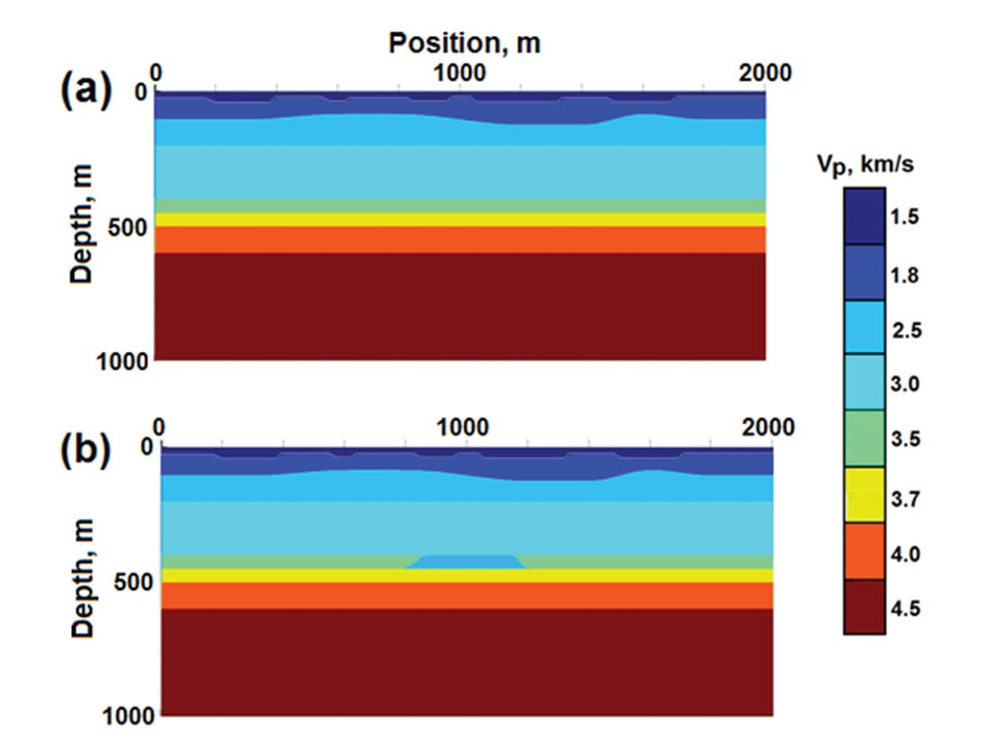
In the first part of the study (Henley et al., 2012), we created a simple plane-layered 2D geological model 2000m long and 1000m deep, with realistic earth parameters, as well as a second model, identical in every way except for a 400m x 50m anomaly zone at 400m depth, where the P and S rock velocities were decreased by about 10%. This is a relatively shallow zone with a strong contrast, which was intended to be easily detected in the absence of noise and other real-world complications. Next, using mFD2D, we created elastic seismic data sets from the geological models, processed the vertical component data, and compared the seismic images. Our results for those first models are shown in Henley et al., 2012; they were used to help establish acquisition/ processing parameters for more difficult, succeeding models.

To make anomaly detection more challenging and relevant to actual field conditions, we created a second pair of geological models, identical to the first pair, except for the near-surface layer, whose velocity was decreased, and whose uppermost portion contained a series of very low velocity weathering pockets of medium spatial wavelength to induce ‘statics’ in the model traces. This pair of models is shown in Figure 1. A final model complication, not shown in Figure 1, was the simulation of random seasonal near-surface changes affecting the acquired data for the monitor model relative to the baseline model.

Model survey geometry

All models were surveyed using a fixed spread of single receivers along the top model surface with a detector interval of 2m. The source was initiated every 10m along this top surface. Each data set consisted of source gathers for all source positions recorded at all receiver locations, and was spatially oversampled relative to the scale of the anomaly, and to the wavelength of the surface weathering anomalies. From these oversampled data sets, other less-well-sampled data sets were constructed by decimation in order to study image resolution issues.

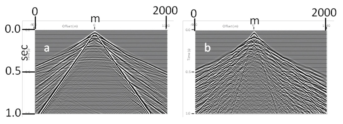
Our earlier analysis of models with no near-surface complexity (Henley et al., 2012) allowed us to determine basic processing parameters for comparing monitor and corresponding baseline surveys. For the more realistic models in Figure 1, the shallow low-velocity layer supports strong source-generated surface and refracted waves, and the weathering pockets at the surface cause not only ‘static’ shifts in the observed traces, but also scattered surface and refracted waves. The strength and bandwidth of surface and near-surface guided waves is controlled primarily by the overall layer thickness and velocity contrast at near-surface boundaries, while static delays are created by variations in the thickness and velocity of the weathered layer itself. Figure 2a shows a vertical component source gather corresponding to the baseline model in Figure 1, but without the weathering anomalies, while Figure 2b shows a vertical component source gather from the same baseline model, but including the weathering. Due to the strong direct and scattered surface wave noise, the underlying reflections visible in Figure 2a are not visible in Figure 2b. Sets of 2D elastic seismic source gathers like that in Figure 2b were created for both the baseline and monitor geological models portrayed in Figure 1, and strong bandlimited random noise (rms S/N = 1.0) was added to all the traces to further increase processing difficulty (noise not shown in Figure 2b).

A final complication added to the modeling experiment for the example shown here was the simulation of seasonal variations in the near-surface by adding random statics to the monitor model data. The simulation was performed by picking a fictitious ‘jittery’ horizon across a source gather for the monitor survey, then a similar uncorrelated ‘jittery’ horizon across a monitor survey receiver gather. The jitters were created with hand-picking and were as random as possible, but never exceeded approximately 10-15ms. The ‘jittery’ horizon picks were turned into surface-consistent statics by first applying the individual source-gather pick times (minus their mean value) to their respective traces on each source gather, sorting the data set to receiver gathers, and then applying the individual receiver-gather pick times (minus their mean value) to the respective traces of each receiver gather. The incorporation of these ‘seasonal variation’ statics into the monitor model data meant that we could not simply re-use a residual statics solution from the baseline model for the monitor data – the solutions had to be computed and applied independently.

We applied identical cascaded radial trace filters to all the source gathers in both data sets to attenuate the coherent noise (Henley, 2011). We then used Gabor deconvolution on individual traces to broaden the signal spectra in the presence of the added random noise. NMO stacking velocities were determined by interactively fitting hyperbolas to reflection events on displays of the de-noised and whitened baseline source gathers; the same velocities were then used to correct both data sets for NMO.

Autostatics results

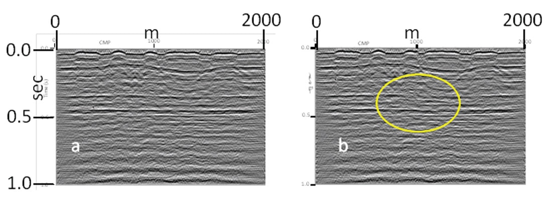
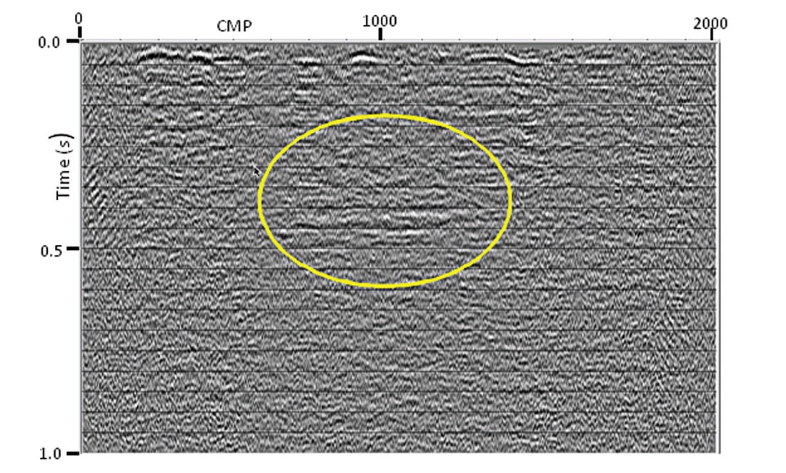
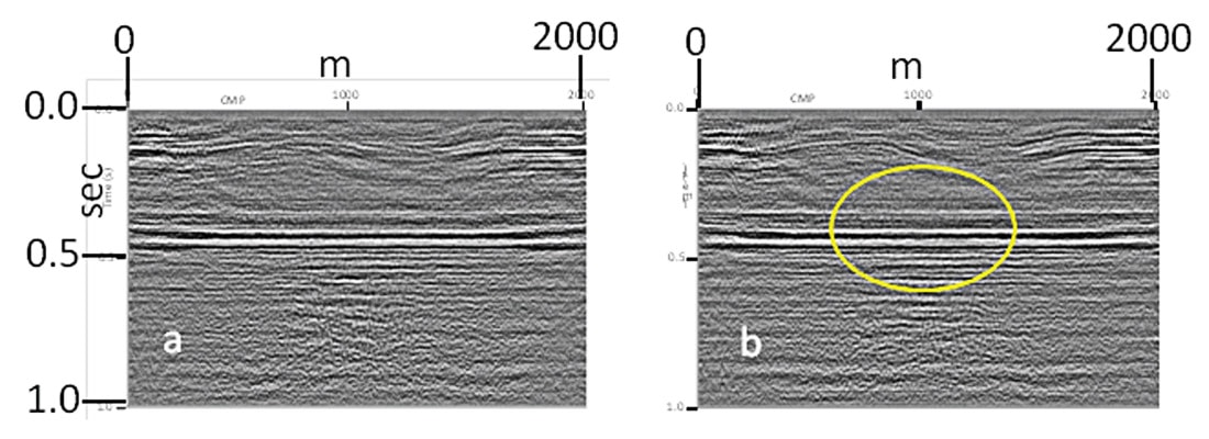
Residual static corrections were computed and applied to the traces of each model before CMP stack in order to obtain sufficient stack power and coherence along the reflection events to detect amplitude/time anomalies between baseline and monitor surveys. We chose to use a ‘maximum-stack-power’ autostatics algorithm (Ronen and Claerbout, 1985), but found that considerable parameter experimentation was required for success, because of the high level of random noise (which degrades the cross-correlations used in autostatics algorithms). It proved necessary to apply three consecutive passes of autostatics in each case, in order to obtain an acceptable statics solution. Figures 3a and 3b show the CMP stacks of the noisy baseline and monitor models, each after three passes of autostatics, while Figure 4 shows the arithmetic differences of the stack images. Since the autostatics program was run independently for each model, Figure 4 shows image differences not only due to the time-lapse anomaly, but also due to the differences in the autostatics solutions near the surface, probably caused by the seasonal variation simulation. Note that the uppermost visible time-lapse anomaly event at about 400ms is an actual event amplitude difference, while the deeper anomaly is more likely due to timing mismatch or ‘sag’ of a reflector beneath the actual anomalous zone. The strongest anomalous amplitudes at 400ms are displaced from the centre of the actual anomaly, perhaps due to ‘lensing’ by the undulating shallow interface above.

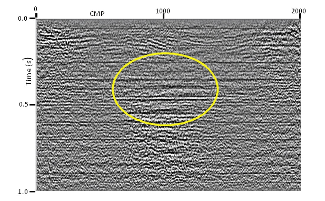
Raypath interferometry results

Recent success with the use of raypath interferometry for applying static corrections to seismic field data (Henley, 2012a, 2012b) led us to apply this technique to our models, since the method is much less sensitive to input parameters and totally insensitive to the actual distribution of statics in the data. Also, unlike autostatics algorithms, the performance of raypath interferometry is relatively robust in the presence of random noise. Use of common wavefield smoothing horizons for both baseline and monitor surveys guarantees the proper time registration of their images for comparison, unlike images with independent autostatics solutions, which may require a small bulk shift to properly register baseline and monitor images. We applied one pass of raypath interferometry to the random-noise-contaminated baseline and time-lapse models. The resulting CMP stack images are shown in Figure 5. The anomaly is distinctly visible in the stack difference image in Figure 6. Interestingly, the top of the anomaly at 400ms is weaker than the time sag anomaly beneath. Its strongest amplitudes are also displaced from the actual centre of the physical anomaly, as in Figure 4. The time sag here is not only more distinct, but affects deeper interfaces, as well, unlike Figure 4. This may be due to an effectively longer lateral wavelength of the raypath interferometry statics solution, compared to autostatics.

Conclusions

We have shown a significant example from a 2D elastic-wave modeling study which we used to explore some repeatability issues associated with the time-lapse technique for monitoring the progress of fluid change in a subsurface formation. Modeling a relatively shallow and strong velocity anomaly, we showed that the detection of time-lapse differences is surprisingly robust under conditions of severe coherent and random noise contamination of the raw data, as long as the survey geometry remains the same for both baseline and time-lapse surveys, and as long as identical processing flows, with identical parameters, are used for both data sets. Seasonal near-surface variations, simulated as random source statics and uncorrelated random receiver statics, did not materially affect the detectability of the anomaly, as long as the statics solutions for baseline and monitor surveys were derived and applied independently. Raypath interferometry proved easier to apply for residual statics because of the insensitivity of its parameters to the actual statics distribution; and the resulting anomaly image showed the anomaly-induced time sag of underlying events more clearly than the image prepared using autostatics.

Our original report showed that receiver spacing could be increased to 10m without affecting the detectability of the anomaly on models with a simple near-surface layer; but we found that the complex near-surface layer in the models shown here required the high-fold 2m receiver spread to provide sufficient redundancy for successful imaging.

Acknowledgements

The authors acknowledge the support of CREWES sponsors and NSERC grant funds, as well as Landmark/Halliburton for supplying the ProMAX software package.