True Depth Conversion: More Than a Pretty Picture

A good seismic image is not enough for an exploration or field development interpretation. Good well ties and reliable depth conversion are also required. The authors have found that geologists and geophysicists tend to approach the depth conversion process quite differently. The geologist says, “If I don’t have wells, how can I do depth?” - often unaware that seismically-derived velocities exist. The geophysicist says, “I have all these velocities from my seismic,” - and needs to be cautioned that these imaging velocities are not right for true depth conversion.

We have also seen that there is sometimes confusion about what the deliverables of a depth conversion project are. These can be 1) seismic data volume (SEG-Y) in depth instead of time, 2) maps and/or computer grids of depth from the seismic and wells, 3) a velocity model in the form of a 2D profile or 3D cube data volume (SEG-Y), 4) another possible deliverable is an uncertainty analysis on the final ‘best’ result.

Recently we have also seen confusion over the meanings of “depth migration” and “depth conversion,” which are two different processes. Migration is an imaging issue; conversion is a calibration issue (although some blurring of the lines has arisen recently with the advent of anisotropic, pre-stack depth migration, or APSDM). The differences are discussed later in this article.

This article will describe various methods to perform depth conversion, including how much sophistication is needed for various objectives. We will discuss accounting for real geologic structure and stratigraphy, proper calibration of seismic velocities, proper honouring of well data versus seismic data, and suitability to meet time and cost constraints.

First things first: why depth?

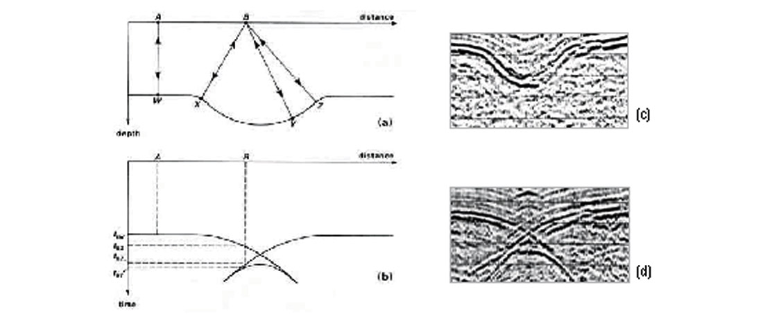
One thing there is no confusion about is that subsurface rocks exist in depth. Seismic reflection data portray this subsurface in recorded two-way time. Most seismic interpretation is done in the time domain, which is quick and is acceptable for many situations. Stratigraphic interpretation in the time domain is usually fine for seismic facies and sequence stratigraphy analyses, because their interpretation remains largely the same with changing structure. Structural interpretation in the time domain is a riskier business. Interpreting structure in the time domain means accepting the risk of assuming a constant velocity model, or that all possible velocity aberrations can be caught by the interpreter. Further, even simple geology can produce false highs (or can obscure true highs) - a ‘velocity anomaly’ is not required in order to have a time structure. A thick zone of high velocity material can masquerade in the time domain as an evenly deposited layer of rock overlying a structural high (Figure 1). Many good interpreters have fallen into this classic pitfall! Similarly, structures can be concealed by the overburden, and a good depth conversion can show structures where none were thought to exist, revealing potentially bypassed reserves.

Depth conversion is a way to remove the structural ambiguity inherent in time and verify structure. Explorationists need to verify structures to confirm the presence of a structural trap when planning an exploration well, or to determine the spill point and gross thickness of a prospect to establish volumetrics for economic calculations, or to define unswept structural highs to drill with infill wells to tap attic oil.

What’s more, there is an increasing use of seismically-derived rock property data in reservoir studies. Geological and engineering reservoir modeling studies are inherently in depth. By translating seismic interpretations from time to depth, we enable the integration of the seismic asset with geologic, petrophysical, and production data.

There are many methods to convert seismic times to depths, too many to cover in one article. Depth conversion methods can be separated into two broad categories: direct time-depth conversion, and velocity modeling for depth conversion. Whichever method is selected, an accurate and reliable depth conversion is one that will 1) tie the existing wells, and 2) accurately predict depths at new well locations.

A word to the geophysicist: imaging is not depthing

Recognizing that simple vertical ‘stretching’ of seismic times to depth cannot correct for lateral position errors that may be present in the seismic image, we must ensure that a suitable image be produced before we attempt a depth conversion. This is largely an independent step from the depth conversion, and is called ‘imaging’. Imaging addresses the proper focusing and lateral positioning of reflectors. Depthing addresses the vertical positioning of seismic times to true depth, using true vertical propagation velocities.

Although both imaging and depthing require velocity, the type of velocity used is different (Al-Chalabi, 1994; Schultz, 1999). Imaging uses velocities designed to flatten gathers during stacking, or derived from migration. (Here the authors adopt the terminology of Al-Chalabi (1994), who suggests the term “provelocities” to refer to imaging velocities obtained from seismic processing.) Depthing, on the other hand, requires true vertical propagation velocities, such as are obtained from well measurements (Table 1).

A depth conversion consists of imaging first, to obtain the best image, then depthing, to tie wells and predict depths away from the wells.

“I did a depth migration, haven’t I converted to depth?”

This commonly asked question is a good one because it forces us to examine our understanding of imaging. The truth is that depth migrated data sets are not depth converted.

Whenever the subsurface layers that we are trying to image seismically are not flat-lying, the reflected image we see on an unmigrated section will not correspond to the real position of the structure.

On the unmigrated seismic section, for example:

• The observed dip of a sloping reflector will be less than the true dip.
• Synclines will appear narrower than they really are.
• Severe synclines will appear as ‘bow-ties’.
• Anticlines will appear wider than they really are.
• Any abrupt structural edge acts as a point scatterer and will appear as hyperbolic diffraction.

Migration is a seismic processing step to reposition reflections under their correct surface location (Figure 2).

Migration collapses diffractions. Migration puts the reflected energy back where it came from.

These simple geometric examples listed above show that the need for migration arises when reflectors are dipping. The need for migration also arises when the subsurface velocities vary laterally, as variations in velocity will also cause reflections to be recorded at surface positions different from the subsurface positions.

Time migration is strictly valid only for vertically varying velocity; it does not account for ray bending at interfaces. Depth migration accounts for ray bending at interfaces but requires an accurate velocity model. Depth migration is typically called for when there is significant lateral variation of velocities.

Imaging addresses the proper lateral positioning of reflectors, but does not result in a true depth data set, even if depth migration is used (Al-Chalabi, 1994; Schultz, 1999). Depth migration ‘depths’ often mistie known well depths; errors of over 100 metres are still common after depth migration (Haskey et al., 1998). The “depth” in “depth migration” is not true depth. Why? Because provelocities, those that do the best job of NMO and migration, are not the same as true vertical propagation velocities. Seismic energy, after all, does not travel vertically. There is a strong horizontal element to the travel path of energy that we record in any seismic surface data (Reilly, 1993; Schultz, 1999). Even if you do a zero-offset survey, and you send the source signal down vertically, the raypaths refract in accordance with Snell’s law whenever velocity variations are encountered. Because of Snell’s law and ray-bending, the signal that departed vertically will be unlikely to travel vertically. It is compelled to travel along at directions that are bent away from vertical.

Nonetheless, provelocities are the right values to use for imaging. What makes them so fit for their purpose, though, makes them unfit for the purpose of true depth conversion, because they are designed to correct a different problem. You neither want to use vertical propagation velocities to do depth migration, nor use provelocities to do depth conversion (Table 1).

Is this unsettling? Intuitively, geophysicists feel that there must be an actual velocity at which the seismic wavefront travels through the ground. Over the years, though, velocity terminology has suffered casual use and often misuse.

Unfortunately, what is commonly called ‘velocity’ obtained from seismic processing:

“has the dimensions of velocity but is generally or only remotely or vaguely related to the actual velocity in the ground. The most common type of such ‘velocity’ is what in the industry is commonly known as stacking velocity. ... Its real significance is that it is the parameter that produces optimum alignment of the primary reflection on the traces of the CMP gather, purely that. Similarly, ‘velocities’ obtained via pre-stack migration velocity analysis techniques are primarily parameters that produce optimum imaging of migrated energy. In general, they are quite unrepresentative of velocity in the ground.” (Al-Chalabi, 1994, p. 589)

Transverse isotropy (seismic waves traveling horizontally through a geologic layer will normally travel at a higher velocity than a similar wave traveling vertically) is often the cause of the disparity between the best depth-imaging velocities and the best depth-conversion velocities (Schultz, 1999). Provelocities are generally very different from the true vertical velocity field. For this reason, pre-stack depth migration (PSDM) does not provide the correct depth of events and should just be used for lateral positioning, not for depthing (Al-Chalabi, 1994).

Depth migration output is in the depth domain, but does not result in accurate depths of reflectors because the velocities used are provelocities. This is why depth migration results do not tie wells accurately. Schultz (1999, pp. 2-7 and 2-8) says:

“Even though velocity model-building and depth imaging create a seismic depth volume, their main contribution is an improved image. The depth rendering, via the [imaging] velocity model used for depth migration, is not sufficiently accurate to tie the wells. A major reason for the misties is velocity anisotropy. The migration velocity analysis measures the horizontal component of velocity, and the depth conversion requires the vertical component of velocity. The horizontal component is often faster, and commonly makes the well depth markers come in at a shallower depth than the corresponding seismic reflection event.”

Another reason for the mistie is nonuniqueness: there are many velocity models that will produce an equivalent image (Tieman, 1994; Ross, 1994). Even in totally isotropic media, therefore, unless well data are incorporated into the velocity model (Alkhalifah & Tsvankin, 1995), there will probably be misties - especially due to the tendency to pick on the fast side when picking processing velocities so as to discriminate against multiples.

A good approach to depth conversion, especially in a complex geological environment, is first to perform a depth migration with a velocity model optimized for structural imaging, second to render the resulting laterally positioned depth image to time using the provelocities, and finally to convert the depth-migrated seismic data - now in the time domain - to true depth using a true vertical velocity model (Schultz, 1999; Crabtree et al., 2001). (Figure 3).

Perhaps ‘Depth Migration’ should more accurately be called ‘Lateral Imaging Migration’ - food for thought.

To summarize: imaging first, to accomplish lateral positioning; then true depth conversion using vertical propagation velocities.

Depth Conversion Methods

Once a suitable seismic image is obtained, the depthing step can commence. There is no single method by which this is done, but rather many methods exist and are in use today, not all of which are published in the literature. Each method has its own advantages and disadvantages, and the choice of method is often a subjective one, or dictated by time and cost constraints. This is because no single method can be shown to be superior in all cases.

Direct time-depth conversion

The simplest approach is to convert a time horizon to depth directly - that is, without regard to the structure of velocity variations. Direct time-depth essentially says, “I know the answer (I know the depth at the well); let me come up with a translation function to predict that answer.” This can consist of applying a fixed translation equation, as regression models do, or a spatially-oriented function, as geostatistical procedures do.

The depths calculated via the direct time-depth conversion method can only be assessed by calculating the prediction error at known well locations (1D), but this is a potentially flawed QC method because the depths being predicted are the ones used to develop the prediction equation in the first place. Even the cross-validation method (common in geostatistics), which witholds a given well from the interpolation and then compares the prediction at the location to the real data, is not fully independent in that all the wells were used to develop the interpolation parameters. The direct time-depth conversion method leaves us with little idea of the validity of the time-depth translation relationship between the wells. We can therefore have only as much confidence in these depths as our well control allows, which is usually weak. Moreover, this method prevents the incorporation of any velocity data from seismic, which may provide valuable additional information between well control.

The authors describe this approach as “direct time-depth conversion” because the velocity modeling step is essentially implicit - that is, velocity is not truly modeled, but rather reduced to a translation function. This translation function is fit so as to result in a predicted depth that either minimizes the error or is back-calculated to tie the well depth exactly. Why is this not truly velocity modeling? Because it is hiding many error factors within this translation function. One of the major causes of error in depth predictions is misties in time between seismic horizons and the corresponding geologic well pick in time. Direct methods hide these errors by forcing the wells to tie, thus altering the velocity provided independently by the well and creating (fudging) a new back-calculated velocity to ensure a correct tie. This means that the translation function is now no longer simply a model of the true velocity in the ground - it is a composite correction factor (Figure 4).

Although direct conversion can be done so as to guarantee exact well ties, which are desirable, the loss of independence means that the reliability of predicted depths where no wells have yet been drilled is compromised.

Velocity modeling for depth conversion

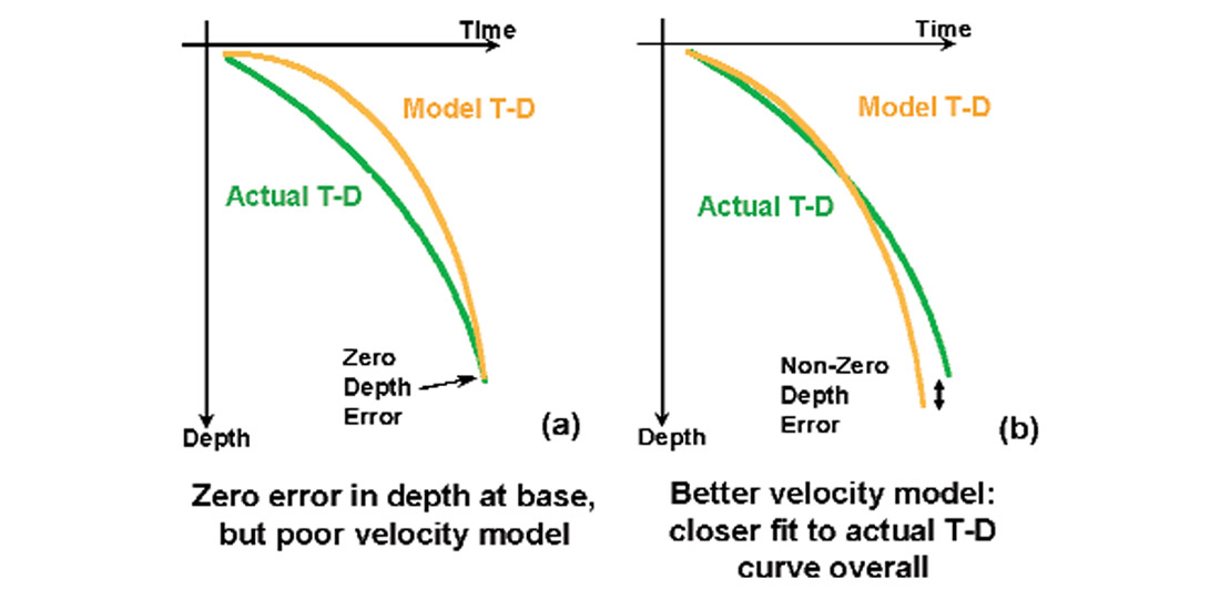
Different kinds of velocity models are required for different purposes (e.g., stacking, migration, depth conversion). When velocity modeling is done as an explicit intermediate step in time-depth conversion, the goal is to derive a robust model that accurately predicts true vertical velocity at and between wells by leveraging knowledge about velocity as an additional tool. In velocity modeling, the description of velocities is the goal, and then the depth conversion falls into place. In direct conversion methods, depths that tie at the wells are the goal, and the velocity is a by-product. In velocity modeling, unlike direct conversion, the ability to predict depth to a minimal or zero error is something that is checked after the modeling, as a test, rather than as a constraint on the procedure itself (Figure 4).

Velocity modeling is a step forward beyond direct conversion because velocity information adds two features to the conversion to depth. First, the velocity model can be evaluated numerically, visually, and intuitively for reasonableness (i.e., tested independently of its ability to predict depth, thus increasing its reliability), something that cannot be done with a global time-depth correlation. Second, velocity modeling enables the use of velocity information from both seismic and wells, providing a much broader data set for critical review and quality control.

Nonetheless, a direct time-depth conversion is often the preferred approach in certain circumstances. It usually offers the quickest solution, and it may be the only one acceptable within the project’s budget or time constraints.

The conversion may only be an intermediate step, intended to be repeated again soon when more data are available. Or, guaranteeing well ties in the immediate vicinity of the wells may be the primary goal of the conversion, regardless of the accuracy away from the wells. From a technical perspective, provelocities may be unavailable, or too noisy or untrustworthy to be of use, and time-depth curves from wells may not be available.

In other words, choice of a conversion method depends partly on the data available and partly on the objectives of the study.

What makes a velocity model robust?

The most reliable velocity model possible is one that is 1) geologically consistent, 2) uses appropriately detailed velocities, and 3) incorporates all available velocity information, weighting different types (seismic and wells) properly.

Geologically consistent means building a velocity model that follows the appropriate layering scheme: in hard rock environments this usually means following the true geological structure, taking into account lithological contrasts (e.g., bedding), folding, and faulting; in soft rock environments the layering may simply parallel the structure of the topography or bathymetry, because velocity may be mainly a function of depth of burial (Schultz, 1999).

In a multi-layer depth conversion, the section is divided into separate geological layers, each of which likely has a different, but internally consistent, interval velocity or velocity versus depth function (Figure 5). A separate velocity model is built for each layer, and results in a depth prediction of the base of the layer, given the top of the layer from the previous calculation. For example, the top of the first layer is usually the seismic datum, then the base of that layer becomes the top of the next layer and the conversion is repeated, layer by layer, down to the last horizon of interest. These layers may not be of exploration interest on their own, but are important because they form the overburden above the zones of interest and may contain significant velocity variation.

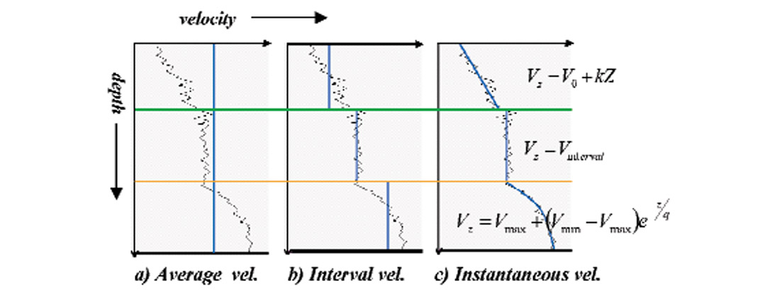
There are three levels of detail in modeling velocity, depending on how the velocity behaves with depth. The simplest level is average velocity, where we ignore the layering and just go straight to the target horizon (Figure 5a). This single-layer approach has the advantage of being simple and quick to implement. The obvious disadvantage is that such a model does not describe the subsurface in detail, so our confidence in the depths predicted may be reduced. There may be good reasons to ignore the detail, though, such as a lack of consistency in the pattern of velocity behavior with depth, or a lack of easily definable horizons.

Adding more detail, we can move on to using interval velocities. Here, we assign a constant velocity to each layer within a given well (Figure 5b). Using average or interval velocities allows spatial variation of velocity between well locations. We can accomplish this by cross-plotting interval velocity versus midpoint depth, for example, or we can contour our well average or interval velocities – perhaps contour them geostatistically using seismic processing velocities at distances far from the wells.

Adding still more detail, we would like our model layer velocities to include variation with depth in some cases, because velocities often increase with greater degrees of compaction caused by thicker overburden (Figure 5c). For these situations we wish to have an instantaneous velocity data set to model, such as a time-depth curve from a vertical seismic profile, or check shot survey, or an integrated sonic log. This type of curve provides velocity variation over very small depth increments, hence “instantaneous” velocity.

The simplest way to describe such variation is to model instantaneous velocity as a linear function of depth: V(z) = V₀ + kZ, where V(z) is the instantaneous velocity at depth Z, and V₀ and k are the intercept and slope of the line. Numerous other functions have also been proposed (Kaufman, 1953; Al-Chalabi, 1997b), some linear and some curvilinear. These functions are fit separately for each layer to ensure geological consistency. The authors advocate using the simplest model that fits the data acceptably well. So, interval velocity is used where appropriate (i.e., no consistent increase in velocity with depth), then preferably a linear model, and finally a curvilinear model only if necessary.

Instantaneous velocity modeling

For those cases best suited to a velocity versus depth function, the issue arises of how to choose the best function. A simple way to check the correctness of a V(z) function is to calculate the depth it predicts for a given geologic top at a well location, where the top depth is known. However, it can quickly be seen that many different V(z) models will calculate the correct depth of a given geologic marker. Which is the best V(z) from among the possible candidates? The best one is the one that will effectively predict depths at locations away from the wells, which is the one that best fits the actual V(z) curve over the entire depth range for the given layer, not just the one with the best tie at the well (i.e., the base of the geological layer) (Figure 4b). But how can we evaluate goodness of fit? There is a unique quantitative method for determining the accuracy of the fit of the models. The authors call this approach “discrepancy analysis.” It was derived and patented by Al-Chalabi (1997a), and has been used extensively for several years. What follows is a discussion of Al- Chalabi’s approach.

This approach makes use of the fact that most analytic expressions of velocity variation with depth, whether a linear or curvilinear expression, have two parameters. (The ideas presented here are extendible to functions with more than two parameters. For simplicity, the two parameter case is discussed.) For example, in the commonly used linear equation of the form V(z)= V₀ + kZ, the two free parameters are V₀ and k. Within a given rock layer, the variation of velocity with depth can be described equally well by a range of V₀ and k parameter values. These analytic functions describe a smooth variation of velocity with depth, much smoother than the high frequency fluctuations observed on sonic logs (Figure 6).

In practice no analytic function could represent the actual high frequency flutter of instantaneous velocity with depth precisely - nor should it, because its purpose is not to describe the geology in that specific well, but rather the typical velocity within the geological unit overall. The goal is not to find a function that is an exact fit to the velocity vs. depth data for that layer for any one specific well; the goal is to find a specific parameter combination that produces a closer fit than any other combination for all wells, and that fits the real functions adequately. How do we assess which parameter pair is the best to use, among the range of possible parameter pairs?

The goodness-of-fit between the well velocity data and the calculated function curve can be calculated. Both parameters are varied and the goodness-of-fit calculated for each pairing, which is termed “discrepancy.” The value of the discrepancy at each parameter pairing is given by

where V_i and C_i denote the i^th actual (observed) and function velocity values respectively, m is the number of sampled depth points, and q is the norm (q=2 in this case).

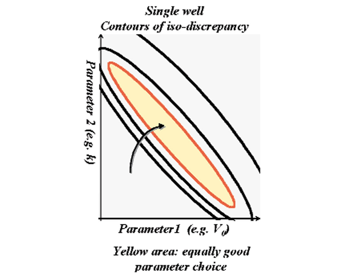
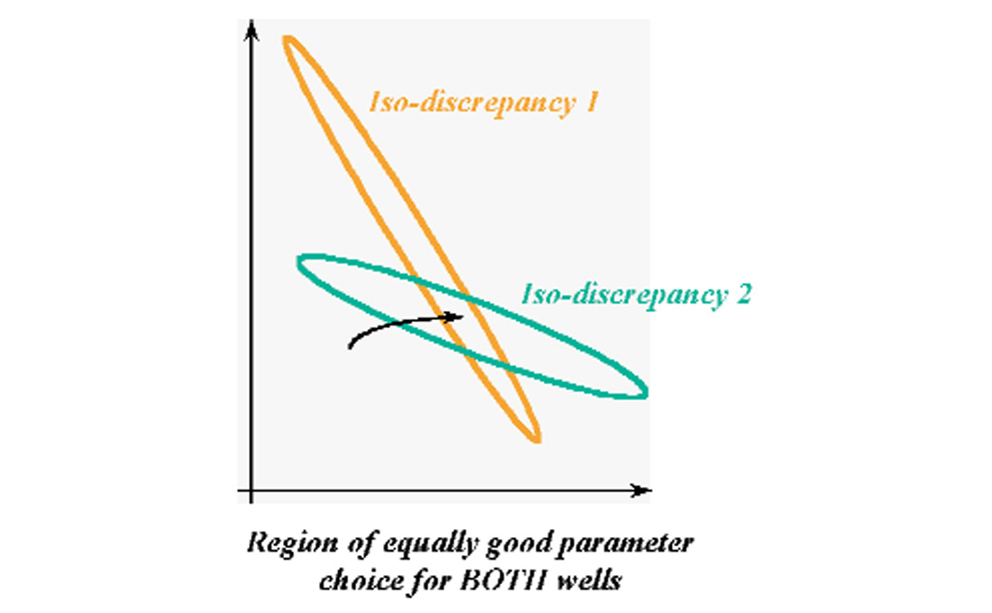
In the crossplot space of the two free parameters (V₀, k), the discrepancy values for each pairing are contoured. Each iso-discrepancy contour delimits a region in the parameter space inside which any (V₀, k) combination produces a function that fits the well velocity data more closely than the value of that de-limiting contour. The area within an iso-discrepancy contour is an area of equally good parameter pairs. The discrepancy contour corresponds to a margin of tolerance. (Figure 7)

There is no single parameter pairing that can be considered the ‘exact’ solution, especially where a single well is concerned. A given parameter combination may, however, satisfy the data from more than one well. By making a composite discrepancy overlap plot of the discrepancy contours for the same layer in two wells (or three wells, or many wells), the region of overlap between the contours represents the (V₀,k) pairs that would produce a V(z) function that would fit both wells to within the appointed margin of tolerance. That is, any such parameter combination would provide a single function that applies to the whole area adequately and correctly. Through the use of discrepancy overlap plots the range of acceptable parameter pairings can be reduced, thus increasing the confidence in the applicability of the parameters over a large area. (Figure 8)

If a single region of overlap can be found, then the reliability of the model is high since it applies to all wells used in the analysis. Thus, predicted values between the wells should be reliable. If the wells don’t all overlap, but instead break into clusters (Figure 9), it may indicate that there are several different sub-areas within the overall area. These are often different fault blocks, or different facies associations. These situations can be handled by holding one parameter constant, such as k, and then solving for the other, allowing it to vary. Once calculated for all wells, it can then be mapped, providing a map of anticipated differences in uplift or facies.

The discussion thus far has focussed on calculating velocity models from wells. The patient reader has been waiting for the discussion to open up to the possibilities that seismic data offer to velocity modeling. The despairing reader may even have seismic but no well data. Are the benefits of velocity modeling still available in this situation? The following sections show that velocity modeling, including instantaneous velocity modeling, is still available even when only provelocities are available.

Use all available velocity data to build a robust velocity model for depth conversion

While no-one would disagree with the advice, “Use all available data”, we must bear in mind that different types of data have different degrees of certainty, particularly well data versus seismic data. Well data can consist of vertical seismic profiles (VSP), check shot surveys, sonic logs, or some combination of these in several wells. VSP and check shots may be used directly, but sonic logs require corrections for “drift” to be comparable to a VSP or check shot survey in the same well (Reilly, 1993). Generally speaking, VSP are preferred most, then check shots, then integrated sonic logs, but the more wells available the better, even if it means mixing different types of time-depth curves.

Well data are hard measures of depth - not completely without error, but the well depth measurements carry relatively low uncertainty. However, wells present us with velocity information that is spatially sparse, often clustered, and limited by well total depth. Further, well data overrepresent anomalous locations, such as structural highs. Seismic data offer a spatially dense, regular, and objective sampling, and cover the entire depth range evenly throughout the survey area. These traits offer the opportunity to overcome many of the limitations of using well data alone. However, seismic data are a measure of time rather than depth or velocity directly, and the provelocities derived from seismic are imaging velocities, not vertical propagation velocities such as in wells.

Any effort that undertakes to combine hard (well) data (high certainty and low sampling density) and soft (seismic) data (low certainty and high sampling density) must honour the higher certainty of the well data. Geostatistics (spatial statistics) is the proper way to combine these two diverse types of data and retain proper weighting of well control, as well as to capture and maintain spatial trends (Chambers et al., 2000). For instance, kriging (which here is taken to include the various versions of kriging and cokriging) is a method of interpolation that uses specially-weighted combinations of data observed at known locations (such as wells) to predict unknown values at other locations. Kriging also provides estimates of the accuracy of the predicted values.

The field of geostatistics presents many interesting techniques for integrating and mapping velocity, and analyzing spatial structures of velocity. We must restrict the scope of this short article to the topic at hand - depth conversion - and simply note that geostatistical analysis offers us tools to combine all available velocity data.

Extending the velocity model to make use of velocities from seismic

How can we extract good quality vertical propagation velocity information from seismic data? Recall our earlier discussion that the provelocities used in processing the seismic data to a stacked, migrated, laterally focused picture of the subsurface reflectors are not the same entity as true vertical propagation velocities in the same ground, which are what we require for depthing. We can correct them substantially, however. The provelocities require corrections for anisotropy (depthing demands the vertical velocity, and provelocities contain a horizontal velocity element), for heterogeneity (due to lateral facies changes and such), and for ray bending (Al-Chalabi, 1994). These corrections produce closer estimates of the true vertical velocities for accurate depthing.

Although provelocities will always have more error and uncertainty than well velocities, we can at least calibrate them to the wells and then benefit from their added spatial coverage. Calibrated provelocities can be converted either to average or to interval velocities, and then combined with well average or interval velocities, preferably using an appropriate geostatistical approach (e.g., kriging with external drift, collocated cokriging, etc.). This approach is often very useful in the first layer of a multi-layer depth conversion, where instantaneous well velocities are often limited or absent (due to no logging behind surface casing), and where average provelocities handle the overburden and provide extensive, unbiased areal coverage.

Perhaps more usefully, though, provelocities can also be used for instantaneous velocity modeling, using several different approaches. In one such approach, well data are used to derive the gradient parameter (k) in the V₀,k function, and interval velocities extracted from seismic and converted to V₀ are used in combination with well V₀ values in a V0 map. Another approach is to derive the V₀ from the provelocities after they have been converted into “pseudo wells,” described next.

The advantage of these approaches is that the wells provide the necessary detail in the vertical direction (k gradient), the seismic provides the necessary detail in the lateral directions (V₀ map), and geostatistics ties them together with proper spatial weighting.

Pseudo-wells from seismic

One of the unique things that can be done with provelocities is to compute “pseudo-wells.”

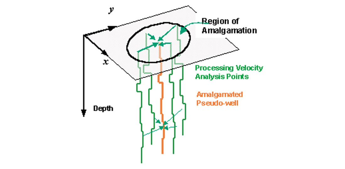
From provelocities that have been calibrated to true vertical velocities, time-depth curves (T-D curves) are computed at each stacking location. (T-D curves are just another way of representing velocity-depth functions.) Then T-D curves can be amalgamated (averaged) into pseudo-wells to be used in instantaneous velocity function modeling just as the T-D curves from wells are used for instantaneous velocity modeling, albeit at a coarser time sampling (Figure 10). The averaging is used to smooth the error inherent in stacking velocity analysis.

It can quickly be seen that even if we have seismic only and no well data or sparse wells, we can derive pseudo-wells and do instantaneous velocity modeling for our depth conversion. In this way we can use V(z) gradient functions to model velocity even if we are using seismically-derived velocities. In order to do this, though, seismic velocities need to be sufficiently detailed vertically to allow a robust V(z) curve to be derived. An approach to pre-stack velocity analysis has been developed to produce “geologically consistent velocities” in seismic processing (Crabtree, et al., 2000). In addition to providing a finer spatial sampling along the time axis, this technique forces a closer fit to well velocities and generally reduces the artifacts that are typically present in provelocities.

Because of the greater areal coverage of seismic, one of the significant uses of pseudo-wells is to create many wells spread out across a study area and perform discrepancy contouring and overlap plots to look for clustering of pseudo-wells into areas of different velocity behavior. This points out areas of major facies changes or differences in uplift caused by faulting. The pseudo-well technique is a geological tool as well as a velocity modeling tool for time-depth-conversion. It can be used for the detection and evaluation of anomalously-pressured geological units, such as geopressured units (Gordon et al., 2000) that must be dealt with during drilling (or avoided), and basin-centered gas accumulations (Surdam, 1997).

Summary

In this article we have touched on a number of issues with regards to translating seismic from time to true depth. Seismic imaging is a separate step and must be addressed before depth conversion. No depth conversion can correct for improper lateral positioning of events, because depth conversion is a vertical process only. Depth migration is currently the ultimate tool for lateral imaging, but it does not calibrate the seismic to true depth, because it does not use true vertical propagation velocities. This is not an error - imaging is a separate issue from true depth calibration.

All imaging processes use a category of velocity that is more properly called “provelocity,” although “imaging velocity” or “seismic velocity” suffice as well. Provelocity is appropriate for imaging because seismic acquisition and processing involve both vertical and horizontal velocity to varying extents, but it is inappropriate for depth conversion - or “depthing” - because depthing requires strictly actual vertical propagation velocity (“true” velocity). True velocity is best obtained from vertical seismic profiles, check shot surveys, or calibrated sonic logs.

Depthing can be done via a wide range of existing methods, too many to cover in any article, but which can be separated into two broad categories: 1) direct time-depth conversion, and 2) velocity modeling for time-depth conversion.

Direct time-depth conversion ignores the structure (spatial patterns) of velocity, and operates at known depth points only (i.e., at wells) by forcing an exact or minimal error match between actual and predicted depths. Moreover, direct conversion only involves seismic times at well points - velocity information from seismic, and all the spatial benefits that go with it, cannot be used.

Velocity modeling for time-depth conversion involves building a true velocity model using all available velocity data. This modeling may include various types of well velocities only, or calibrated provelocities only, or both. Modeling may use simple average velocity (single layer), or interval velocity (multi-layer), or instantaneous velocity (variation of velocity with depth). The goal is to determine a model that has some likelihood of working adequately between the known depth points, in addition to matching the known points. Some techniques can be used involving conditions other than final depth prediction accuracy, and can then be tested against the known points to determine their effectiveness. This is an independent way to predict depth because it uses velocity functions as the input rather than horizon depth and time at wells, and because it can involve provelocities in addition to or even instead of well velocities.

The choice of a depthing method depends on data availability and quality, depthing objectives, and time and cost constraints on the depthing process. Direct methods are fast and accurate at the wells, which may be all that is required. Some forms of velocity modeling can also be fast and exact, whereas other forms require significant data resources, modeling expertise, and time to administer, yet offer greater confidence in the results, particularly between well control, where it really counts.