Using uncertainty in quantitative seismic characterization

Over the past two decades, the overall trend has been for a more quantitative use of seismic in building geomodels and interpreting subsurface data. Acoustic seismic inversion has become commonplace, and more complex techniques tend to move closer to a direct modeling of petro-physical properties such as porosity or fluid saturation, through elastic inversion, seismic facies modeling or direct petro-elastic inversion. However, as soon as a numerical answer to a problem is given, it is important to try and analyze the associated uncertainty, as this is the only way to assess the level of confidence that can be given to results.

This uncertainty has been studied in different ways, ranging from a rigorous mathematical framework – such as stochastic inversion – to more qualitative approaches. In this paper, we will show several examples illustrating how uncertainty analysis is not only worthwhile for the accuracy it adds to the models, but also for what it tells about the models themselves, and that even a qualitative approach to uncertainty may bring value to a quantitative model. Further, and perhaps most importantly, tools exist to quantify and properly integrate uncertainties, and this helps communication to flow across disciplines much more easily. For example, when uncertainty in elastic properties can be expressed in terms of properties that engineers are fluent in, such as connectivity, then the integrated workflow is strengthened and made more meaningful.

The first example examines the effect of seismic frequency bandwidth on uncertainty. We know that the increased frequency bandwidth of new broadband seismic techniques provides a much clearer picture. Looking at the uncertainty associated with facies models, we show that this increase in imaging quality does indeed translate to an improved quantitative interpretation, strengthened by facies-probability volumes.

The second example involves rock physics, which seeks to model and establish relationships between a rock’s material properties and the observed seismic expression. Since modeling of petro-elastic properties is very complex and case-dependent, there is a large uncertainty associated to it. However, we show how the use and analysis of rock physics templates enables an increase in the confidence of the results of a petro-elastic inversion to estimate porosity and fluid saturation in a carbonate field.

Finally, we turn to stochastic inversion, which allows to directly produce in a fine scale stratigraphic framework a large number of realizations of impedance matching the seismic data, well logs and specified spatial constraints. The results of this mathematically rigorous approach can then be further interpreted in terms of facies probabilities. In an example in a turbidite reservoir, we show how the connectivity between wells may be assessed in a probabilistic manner.

Reducing the interpretation uncertainty through broadband seismic

One of the biggest intrinsic limitations of seismic data has always been its limited frequency bandwidth, typically from 10 to 70 Hz in marine data. This not only precludes accessing fine scale details, but also makes it difficult to reliably estimate the low frequency trends that are very important to build a reliable petro-elastic model. Broadband seismic uses a combination of specific acquisition techniques and processing to significantly extend the bandwidth in both the low and high ends. This increase is directly visible in the imaging results that are much better focused and detailed. However, it may not be obvious how such an improvement affects quantitative reservoir-scale impedance models.

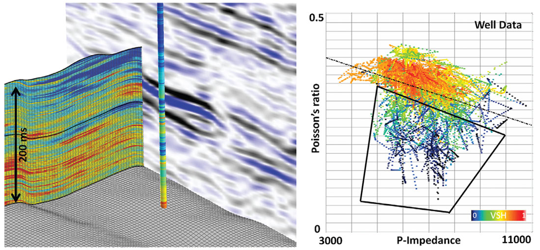
A 2D line was acquired in NW Australia and processed both using conventional techniques and broadband workflow (Soubaras & Lafet, 2013). The target area in the line covers about 25 km, has a thickness of 500 ms to 1000 ms and is intersected by 3 vertical wells. It images a clastic gas-filled reservoir formed of a laterally relatively continuous sand bed, see Figure 1 (left). On the well logs, the reservoir interval is clearly defined on well B, but much less so on well A, so it is interesting to see if inversion of the seismic data allows inter-well prediction, and how this prediction differs between conventional and broadband seismic.

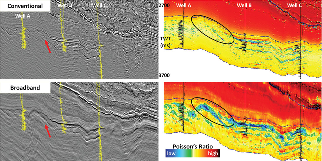
An elastic prestack inversion was run on both conventional and broadband versions, and the results used to generate Poisson’s ratio (PR) sections. Since the purpose of this test is to estimate the difference brought by broadband seismic, the initial model used for both inversions is the same, and is built only from the low frequency trend from the conventional seismic velocity model. As the wells are relatively far apart from each other and are consistent with the velocity model, not using them is not an issue. Figure 1 (right) shows the resulting PR sections. As expected, the results from the broadband seismic look more detailed. Moreover, there is a large anomaly of low PR between the wells, which could be indicative of continuous gas sand. However, from this picture it is impossible to say whether or not the inversion results are actually better.

To estimate the confidence on this prediction, a simple rock physics model is built from a cross-plot of elastic attributes (Figure 2, left). On this plot, well data are color-coded by the observed well facies (shales, water or gas sand). The facies of interest is the gas sand, showing overall a lower PR. From each facies, a probability density function (PDF) is then built: it indicates, in each point of the cross-plot, what are the relative probabilities of being in each of the three facies.

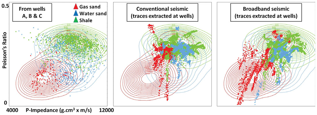
The results of the inversions of both the conventional and broadband seismic data are then compared using these PDFs (Figure 2, middle and right). In each case, samples from the inversion result are extracted along the well trajectories and color-coded by the observed facies. The result of the conventional seismic inversion does reproduce the overall trend of low PR for gas sands, however there is also a lot of overlap with the other facies. On the other hand, the broadband seismic results are much more consistent with the rock physics distribution from the well data. Consequently, the broadband results can be considered as less uncertain, since they are closer to a physical model that was not used to constrain the inversion.

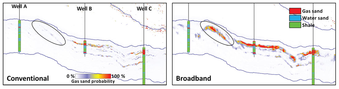
Finally, these PDFs can be used in a Bayesian classification scheme (Silverman, 1986; Nieto et al., 2013) to derive probability sections for each of the three facies. Figure 3 shows the gas sand probability for the conventional and broadband seismic data. The broadband result not only confirms the likely gas-bearing sand body in between the wells, but also indicates that the uncertainty on this body is low (its probability is very high), whereas on the conventional seismic the same body appears with a much lower probability, i.e. is more uncertain.

Assessing the confidence in a carbonate petro-elastic inversion

Rock physics is becoming a key element of the geosciences workflow, since it allows to link seismically-derived elastic attributes directly to petro-physical properties such as porosity or fluid saturation. Moreover, the analysis of the available data can provide valuable information on the confidence of an inversion, as shown above. In this second example, rock physics helps in understanding what can be trusted from a direct petro-elastic inversion.

Direct petro-elastic inversion aims at producing directly porosity and fluid saturation from prestack seismic data (Bornard et al., 2005; Coléou et al., 2005). In this case, it was applied to data from a carbonate oil field offshore Brazil (Allo et al., 2011). The target is composed of three grainstone reservoirs, separated by mudstone intervals clearly visible on the seismic. Thin sections show that the reservoir porosity is a complex mix of intra-particle and inter-particle porosities. This complex structure implies a low sensitivity of the elastic properties such as Vp/Vs ratio to fluid effects, which is confirmed by a cross-plot of elastic properties (Figure 4). The distribution of the well data shows a clear relationship between P-impedance and porosity, but a poor correlation between Vp/Vs ratio and water saturation.

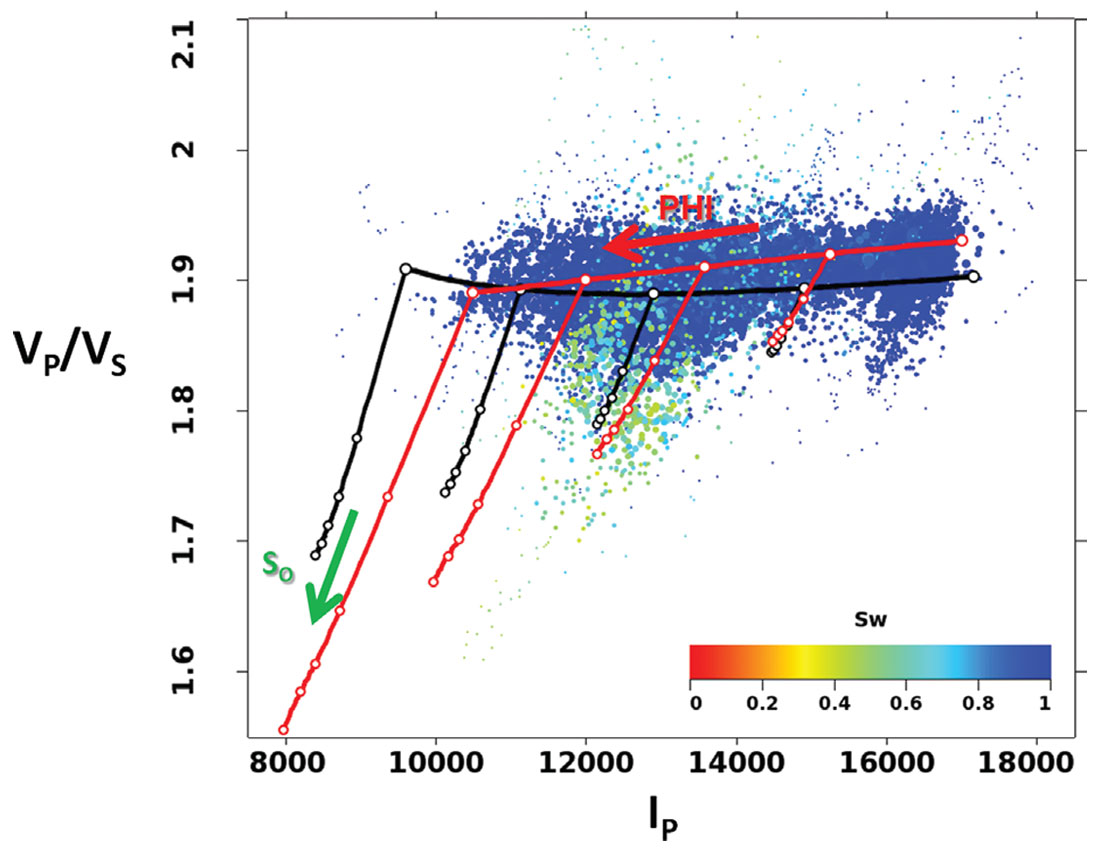
The two most common rock physics templates relative to carbonates can be used to model this data. Both the T-matrix (Agersborg et al., 2009) and Xu-White (Xu et al., 2009) model produce reasonable estimates of porosity, but further show the low sensitivity to water saturation. They can nonetheless be used to try and predict the elastic well logs from the petrophysical ones, as shown on Figure 5. Overall, the Vp log predicted from the rock physics model is very close to the true log, and, as expected, the Vp/Vs log shows little variation.

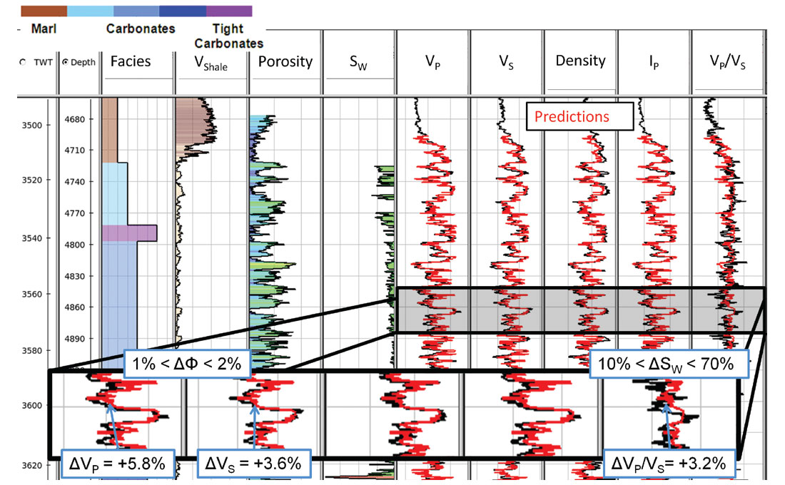
Furthermore, this model can be used to estimate the uncertainty expected on the results of a petro-physical inversion (Figure 5). If one looks at a specific well sample, the error between the predicted elastic properties (Vp, Vs or Vp/Vs) and the measured well log is approximately 3 to 6 %, a reasonably small error. Using the rock physics template of Figure 4 to translate from elastic to petro-physical properties, one can see that for porosity, this translates to a still small error, approximately 1 to 2 %. But for water saturation, the 3 % error on the Vp/Vs translates to an error of anywhere between 10 to 70 %.

Therefore, even before taking the seismic data into account and starting the petro-elastic inversion, it is recognized that although a water saturation estimate will be generated, it will be highly uncertain, regardless of the quality of the inversion itself. This did not prevent us from performing such an inversion, as a careful analysis of the results, in particular the AVO residuals after inversion, still allowed extracting valuable information on the saturations as shown by Allo et al. (2011), but a much better understanding of the reservoir was gained by this study.

Transforming the seismic uncertainty to reservoir parameters: stochastic inversion and connectivity analysis

The previous examples were focused on analyzing the uncertainty for deterministic processes, through the generation of facies probability volumes or qualitative or semi-quantitative error bars. It is also possible to assess the uncertainty in the inversion process itself, by using stochastic inversion.

Stochastic elastic inversion (Buland & Omre, 2003, Escobar et al., 2006) generates a large number of impedance models, or realizations, all constrained by the seismic data, the well logs and some spatial correlation parameters. This robust mathematical framework allows taking into account uncertainties from all types of input data, such as wells, geological property distribution, in addition to the uncertainty on the seismic data itself. The multiplicity of models allows using a fine-scale grid, with a resolution around 1 ms or less, and exploring the uncertainty in the possible elastic models at this scale. This fine scale makes stochastic inversion results very well suited to integration in a reservoir model, since the need for downscaling of the results is reduced.

In this example (Moyen & Doyen, 2009), a stochastic inversion was performed on a turbiditic oil reservoir offshore West Africa (Figure 6, left). The inversion was run in a fine-scale stratigraphic grid with about 180 layers of 1 ms each, and constrained with three wells in addition to the prestack seismic data. The results are several hundreds of P- and S-impedance realizations.

A simple cross-plot of elastic properties at wells (Figure 6, right) is used to transform each realization into a facies model. Sands, with a low shale fraction, are identified from the well logs and a region of interest is drawn on the cross-plot, and finally applied on each realization.

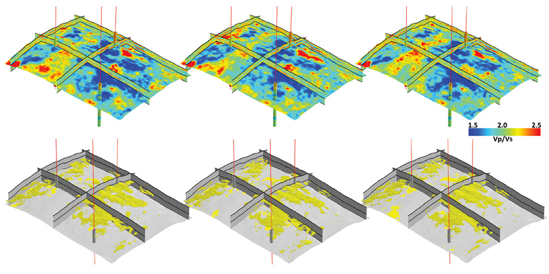
This results in 200 facies models (Figure 7), that can then be summed together to produce a sand probability cube (Figure 8, left). This first result is useful as it shows a large sand sheet between two of the wells, and a highly fragmented sand channel going through the third well, with no connection between the two. It also provides uncertainty information in each point.

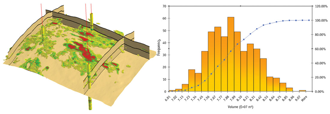
Another way to look at the facies realizations is by computing for each realization the total volume of sand. From this, a histogram showing the distribution of the possible volumes is built (Figure 8, right). This distribution shows the expected range of reservoir volume, and can be used to select quantiles, typically a P10, P50 and P90 (optimistic, median and pessimistic cases). This allows reducing the number of models from several hundreds to a few ones, while keeping the overall variability of the full set of realizations. It is worth noting, however, that this is only adapted if the criterion used to rank realizations (here, the overall sand volume in each model) is representative of the final quantity that is modeled (typically, the oil in place or even the recoverable oil). In this example, this criterion neglects the effect of the connectivity.

It is possible to address this shortcoming and analyze the connectivity in the reservoir. Each facies model derived from a single realization from inversion is processed and connected sand bodies are identified (Figure 9, top-left, Deutsch 1998). Then, the connected sand bodies are filtered so that only the ones connected to the wells are kept (Figure 9, top right).

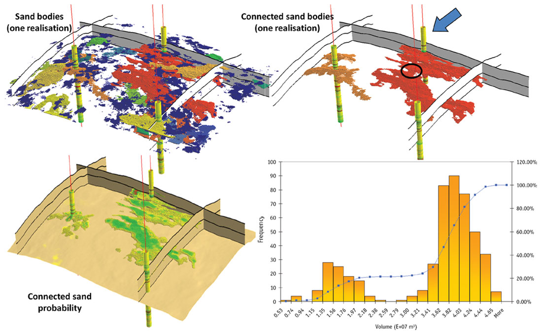
These individual connectivity models can then be summed together. This produces a probability cube of connection to the wells (Figure 9, bottom-left), which clearly shows that one of the wells is not connected at all to the two others, confirming the visual analysis of the sand probability.

More importantly, the connected sand volume can be used as a ranking criterion. This yields a distribution of the connected sand volume across all the realizations (Figure 9, bottom-right). As the connected sand volume is assumed to be a better proxy than the overall sand volume of the dynamic behavior of the model (Hird & Dubrule, 1998, McLennan & Deutsch, 2005), quantiles selected based on this distribution should be more representative of the dynamic uncertainty associated with these seismic-based models.

Finally, this distribution offers a new light on the model. Notably, this is a bimodal distribution, which suggests two very different connectivity scenarios. By looking at a few individual realizations from each of the two populations, it becomes apparent that the difference comes from whether the large sand body situated in the middle (see Figure 9, top-right) is connected to the well at the top of the pictures. This in turn depends on a very small area between the top-most sand body and the middle one. Consequently, the analysis of the uncertainty on the connectivity from the stochastic inversion allows identifying a small area of the reservoir that acts as a bottleneck, and where further fine-scale investigations should be focused. Flow simulation models, for example, are likely to see more influence from whether these two bodies are connected than from the absolute size of the sand bodies themselves.

A similar process was applied on oil sands data (Delbecq & Moyen, 2010). The characterization of the uncertainty, also using stochastic inversion, followed a very similar approach however focused on vertical connectivity instead of lateral connectivity. As in the example shown here, the main idea was to analyze the uncertainty not in terms of elastic impedances, rather in terms of a more reservoir-oriented parameter that was representative of the true challenge of the reservoir.

Conclusions

Through several examples, we have tried to show how uncertainty can be taken into account, modeled and interpreted in quantitative seismic characterization workflows. Although a rigorous assessment of the uncertainty is difficult to achieve, these examples show that estimating uncertainty always deepens our understanding of the model and is well worth the effort. This can be either simple qualitative understanding, or more quantitative information, but this will always lead to better informed, and hopefully more accurate, models.

It is also important to note that these uncertainty analyses do not necessarily require the development of new technologies. Although approaches such as petro-elastic inversion or stochastic inversion are fairly new, they are simply tools used to generate information. Most of the knowledge derived from uncertainty modeling can be obtained by a rigorous analysis of the available data at each step of the reservoir characterization workflow. This article focused on only a few types of uncertainties, mostly related to the distribution of the elastic properties and their relation with petro-physical properties. This is but a small part of all the possible uncertainties that should be taken into account, from the uncertainties in the seismic processing to the final geomodel. Of particular note, geometrical uncertainties (such as from imaging, migration, interpretation, or depth conversion) can also have a significant effect and should not be ignored.

Finally, it is clear that analyzing uncertainties at one stage in the workflow is of no value if the knowledge gained is not transmitted to the other actors of the workflow. The transfer of information between geophysicists, petrophysicists, geomodelers, geologists, and engineers is paramount. This is rarely done at present, but many of the tools and techniques mentioned here can be used to help this transmission (for example, an engineer is likely to better understand uncertainties expressed in terms of connectivity than in terms of elastic properties).

Acknowledgements

The author would like to thank all the clients who provided data and the colleagues in CGG who worked on the examples shown here. This article is the result of numerous discussions with many people, especially T. Coléou, F. Delbecq, P. Doyen and R. Porjesz. Many thanks as well to the SEG and the organizers of the Seismic Uncertainty workshop in Banff in July 2013 where this paper was initially presented.