Over the past decade, microseismic (MS) monitoring has become the approach often used to gain an in-situ understanding of the rock’s response during stimulation. Recently, the utilization of downhole monitoring of treatments has provided for an opportunity to investigate the way these fractures develop by examining microseismic events recorded during stimulation. In the Horn River Basin in Northeastern British Columbia, Canada, geophysicists and engineers used microseismic field data and its interpretation to constrain reservoir models. Generally, it was observed that fracture height, width and length vary from formation to formation.
In the presence of uncertainty in reservoir models input data is required for determining best estimate of a value, and probabilistic methods are used. Risk analysis is a technique to quantify the impact of uncertainties on output variables, and to determine a range of possible outcomes. In this paper we use Monte Carlo simulation and probability density functions (PDFs) that describe likely values of fracture half-length as an input parameter into reservoir models. PDFs and Cumulative Distribution Functions (CDFs) are used in this case to provide realistic estimates of stimulation parameters such as stimulated reservoir volume.
Microseismic Interpretation of events provides an upper bound value for fracture half-length in unconventional shale gas reservoirs. Its CDF for each well on a multi-fractured horizontal well pad provides insight on the understanding of what the ultimate fracture half-length could be after pressure depletion and what the implications for well spacing/ placement in pad design are. This allows a probabilistic approach to production forecasting and reserves estimation and to calculate a robust estimate range of EUR and Recovery Factor. This approach differs from previous work that is based on strong collaborative work between geophysicists and engineers.
This article will contribute technically to the knowledge of the unconventional shale oil and gas industry through the integration of geophysics and engineering, constraining analytical models which can be used as quick look first pass into numerical simulation, and estimation of production forecasts and different reserves categories. Furthermore, some of the design considerations of the multi-well pad, surveillance data such as production logs, chemical fluid and radioactive tracer will be addressed, concluding with a discussion of results.
Introduction
The Horn River Basin is located seaward of a barrier-reef system of Devonian age and corresponds to a marine depositional environment (Oldale and Munday, 1994). The region has been affected only by minor tectonic events. The stratigraphic column is mostly a succession of limestone and shale formations with varying mineral content. Muskwa, Otter Park and Evie Lake formations were deposited in the early/mid Devonian. They are made up of shales that are rich in organic content. While uplifted later from the late Cretaceous to Tertiary, these shales have been buried deep enough to generate large amounts of gas and oil. Much of the hydrocarbons migrated to conventional reservoirs but a large amount has also been trapped in low permeability shales.
Microseismic Data Collection and Processing
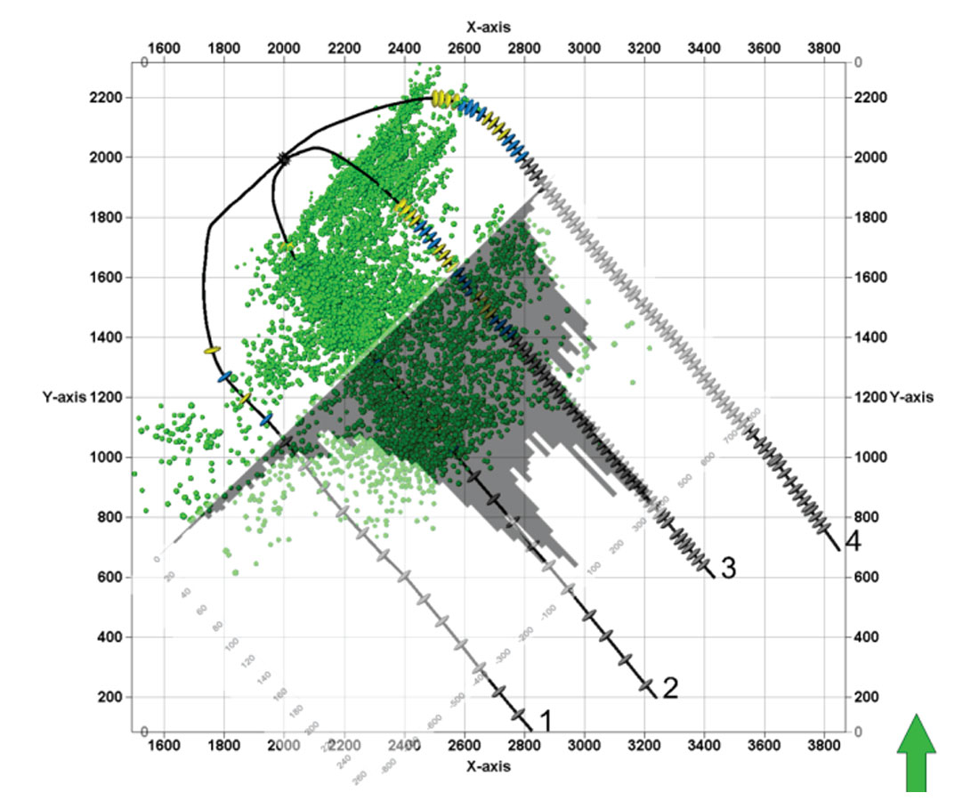
During the completion of an 8 well pad in the Horn River Basin microseismic data was collected. In total 49 stages were recorded from 7 wells locating nearly 40,000 events over a period of 12 days. Figure 1a highlights the perforation locations of the stages recorded by microseismic in blue and yellow. Acquisition of the data was done with a variety of arrays including vertical, horizontal and whip downhole arrays as well as a surface array to accurately locate all microseismic events associated with the hydraulic fracturing.
The borehole seismic data was processed using multiple arrays to increase location accuracy. Perforation shots were used to calibrate the initial velocity model made from sonic logs in the area and included VTI anisotropic parameters. Figure 1b shows the locations of all microseismic events recorded during the completion of the pad.
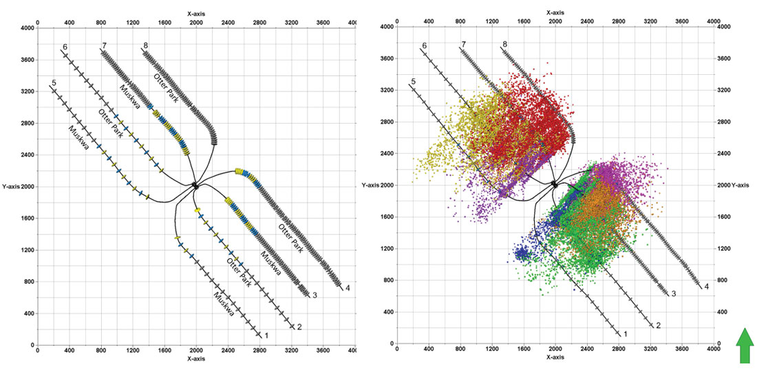
Figure 1b (right). Microseismic event locations.
Microseismic Geometric Analysis
As shown in Figure 2a each microseismic event has associated spatial coordinates. x, y and z UTM coordinates of an event can be converted into R, hf and xf with respect to its stage. R is radial distance to midpoint of stage; hf is vertical height above or below midpoint of stage and xf is the horizontal distance on either side of the wellbore from the midpoint of the stage. Each event also has recorded time, which can be converted to time after breakdown.
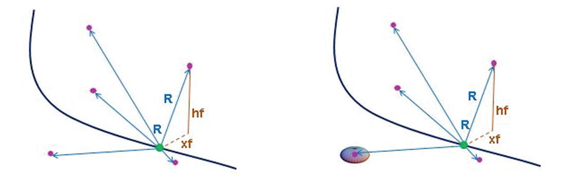
Figure 2b (right). Ellipsoidal shape of microseismic location error.
Data Uncertainty
Microseismic event locations inherently have some uncertainty associated with them, for the pad of interest these uncertainties on average are about 10 m vertically and 20-40 m laterally. Positional uncertainty has an ellipsoidal shape as shown in Figure 2b. Uncertainty is defined as the amount by which a point’s true location may differ from the reported location. Uncertainty varies because the precision of locating the event increases as the event distance from the receiver array decreases.
Probability and Statistics – Histogram Analysis
A histogram is a graphical representation of the distribution of data. It is an estimate of the probability distribution of a continuous variable (quantitative variable). The language used to describe the patterns in a histogram in this paper are symmetric or unimodal and asymmetric or bimodal. Unimodal histograms have one mode, in contrast bimodal histograms will have 2 modes.
A histogram may also be normalized displaying relative frequencies. Histograms give a rough sense of the density of the data and often for density estimation: estimating the probability density function of the underlying variable. A histogram can be thought of as simplistic density estimation, with smoothed frequencies over the bins.
In probability theory, a probability density function (PDF) of a continuous random variable is a function that describes the relative likelihood for this random variable to take on a given value. PDFs may be used when the probability distribution is defined as a function over general set of values, or it may refer to the cumulative distribution function (CDF), which describes the probability that a real–valued random variable x with a given probability distribution will be found to have a value less than or equal to x. In Figure 3a and Figure 3b it can be seen how PDFs and CDFs for Normal and Log-Normal distributions look like. We have selected the normal distribution for this study and its justification of why can be seen in the discussion of the results.
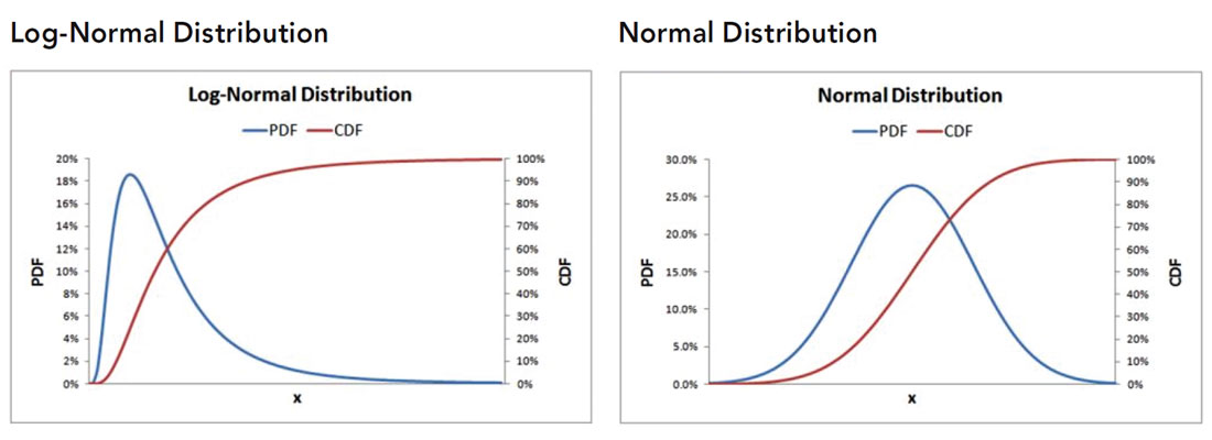
Figure 3b (right). Probability distribution function and cumulative density function for log normal distribution.
Fracture Half-length xf – Use of Probability and Statistics
To analyze the range of microseismic event half-lengths a 100 bin histogram was created for each well. Individual stages were also analyzed however, the results were shown to be less biased by outlier stages when analyzed by well. Figures 4a and 4b show well histograms with unimodal or bimodal pattern for 2 wells that had microseismic recorded.
Proposed Workflow
At the very beginning of the workflow we propose to history match the production and pressure data using a rigorous analytical model based on Stalgorova et al , 2012 where main constrain is microseismic-derived fracture half-length. In this paper we will demonstrate that this microseismic-derived fracture half-length based analytical model will provide the upper bound value for reserves estimation.
Since there are usually multiple combinations of model input parameters that will provide a satisfactory match, the next and final step in the workflow is to run a probabilistic analysis in an effort to assess the full range of uncertainty in the interpretations. The final output includes probability distributions for future production rates, EUR and the associated reservoir characteristics for the expected ultimate microseismic-derived fracture half-length.
Microseismic-derived Fracture Half-length Analytical Modeling
To obtain robust and rigorous long-term forecasts, analytical (or gridded numerical) models are required. It is common to assume that hydraulic fractured stages geometry are bi-wing and planar, however the presence of natural fractures can enhance the region around the main dominant direction of the hydraulic fracture (single perforation) or the complex nature of branching systems. In this paper, a variation of the trilinear model is used. This analytical model (Stalgarova el al, 2012) has three regions: region of dominant fracture conductivity with wide fracture apertures or stimulated complex geometry, region of enhanced stimulated permeability due to presence of natural fractures and unstimulated region where the permeability looks like matrix permeability. The applicability of this analytical model has been demonstrated for high ratios of effective horizontal length and fracture half lengths. A schematic of the modified tri-linear flow model, the enhanced fractured region model and its input parameters and their description is shown in Figure 5a and Figure 5b. In their early study Stalgorova and Mattar (2012) suggested a solution for the case when the enhanced region occupies only part of the space between the hydraulic fractures, but the region beyond the hydraulic fractures was neglected. In their latest study Stalgorova and Mattar considered a generalization that encompasses both the trilinear model suggested by Brown et al (2009) and the Enhanced Fractured Region model presented in 2012.
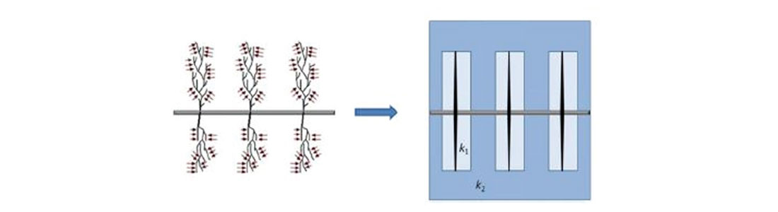
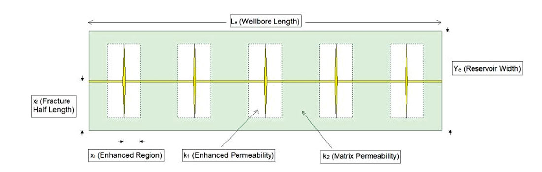
Table 1 indicates the reservoir, fluid and well properties for all wells in the pad
| Well | Le (ft.) | Stages | Clusters | Pi (psi) | T (°F) | H (ft.) | ϕ (%) | Sg (%) | γg | Ye (ft.) |
|---|---|---|---|---|---|---|---|---|---|---|
| Table 1. Reservoir, fluid and well properties for wells. | ||||||||||
| 1 | 5249.3 | 17 | 1 | 4900 | 278.6 | 285.1 | 5 | 90 | 0.66 | 1312.3 |
| 2 | 6233.6 | 20 | 1 | 4900 | 278.6 | 285.1 | 5 | 90 | 0.66 | 1312.3 |
| 3 | 4921.3 | 15 | 4 | 4900 | 278.6 | 285.1 | 5 | 90 | 0.66 | 1312.3 |
| 4 | 6463.3 | 20 | 4 | 4900 | 278.6 | 285.1 | 5 | 90 | 0.66 | 1312.3 |
| 5 | 4593.2 | 15 | 1 | 4900 | 278.6 | 285.1 | 5 | 90 | 0.66 | 1312.3 |
| 6 | 6233.6 | 20 | 1 | 4900 | 278.6 | 285.1 | 5 | 90 | 0.66 | 1312.3 |
| 7 | 5577.4 | 17 | 4 | 4900 | 278.6 | 285.1 | 5 | 90 | 0.66 | 1312.3 |
| 8 | 4921.3 | 15 | 4 | 4900 | 278.6 | 285.1 | 5 | 90 | 0.66 | 1312.3 |
Probabilistic Analytical Modeling
The application of probabilistic methods to analytical modeling allows one to account for uncertainty associated with any of the models input parameters. Unconventional plays are typically great candidates for a probabilistic approach, since most of these wells exhibit linear flow and there is not sufficient data to identify the boundaries of the reservoir. A large degree of uncertainty is usually associated with long, multiply fractured horizontal wells. Variables such as xl , xf , nf , ksrv , km , FCD must be estimated, and it is rare that any of these inputs are known with much certainty.
Analytical models have a large number of input parameters, multiple combinations of which can be configured to match the production history. While two different reservoir configurations may match the history identically, they could produce considerably different forecasts. Instead of manually creating hundreds of deterministic models that match the history Monte Carlo simulation will systematically investigate a defined parameter space and generate probabilistic forecasts. The approach described below accounts for uncertainty in the input parameters, as well as non-uniqueness inherent in analytical models.
Procedure
A deterministic model must first be configured as the base case. This model must possess an acceptable history match, as the quality of the history match will be calculated quantitatively using an average error (see Equation 1) which is used as a cut-off during Monte Carlo simulation.

A forecast must be generated for the base model, the duration and flowing pressure of this forecast will be used to generate probabilistic forecasts. The enhanced fractured region flow model was used as the engine to generate the stochastic results.
Input distributions are specified for uncertain input parameters. Some parameters must be used in regression analysis in order to match the production history. These parameters will be referred to as ‘regression parameters’, they do not require a distribution as their value is determined by the best-fitting algorithm of the analytical model. A Monte Carlo simulation is run, consisting of hundreds of runs. For each run, a value is randomly selected from each input parameter distribution, the regression parameters are re-calculated to match the production history and the resulting forecast and output parameters are stored. Any realizations that do not match the history (according to the specified history match cut-off) are discarded from the results. This process repeats itself hundreds of times, investigating the entire parameter space. Instead of using one deterministic model to describe the reservoir, hundreds of different reservoir configurations and characteristics are evaluated and a range of possible forecasts is generated.
This procedure was applied to all eight wells. One hundred twenty five runs were attempted for each simulation, the objective was to obtain at least fifty to 100 successful history matches per well.
Estimating Input Distributions
Specifying input distributions for all of the input parameters can be difficult in the absence of data. There are hundreds of types of distributions available, however if sufficient data is not available, one is forced to make assumptions. In this paper, the triangular distribution was used for most of the uncertain parameters except for fracture half-length which distribution is defined by the microseismic data. This is a simple distribution that only requires three points. Often times these three points (minimum, most likely, maximum) are known, or can at least be estimated with some degree of confidence. The type of distribution applied usually has a much smaller effect on the results, compared to the range of the distribution. Effort was focused on specifying accurate minimum and maximum values for uncertain input parameters, rather than choosing between distribution types.
Table 2 below lists the uncertain and regression parameters used in the Monte Carlo simulation for all the wells. Similar distributions were applied for all the other wells; however some of the min/ mode/maxvalues had to be tweaked on a per well basis.
| Parameter | Distribution | Min | Mode | Max |
|---|---|---|---|---|
| Table 2. Example of inputs for rate transient analysis – well with cluster perforation. | ||||
| nf | Triangular | 20 | 40 | 80 |
| ksrv | Regression | – | – | – |
| km (nd) | Log-Normal | 5 | 20 | 100 |
| Sg (%) | Triangular | 70 | 80 | 90 |
| Sw (%) | Dependent* | – | – | – |
| hf (m) | Triangular | 55 | 87 | 140 |
| ϕ(%) | Triangular | 4 | 5 | 6 |
| FCD | Regression | – | – | – |
| * Dependent on random sampling of Sg, Sw is re-calculated to ensure saturations sum to 100%. | ||||
Table 3 shows a comparison between the microseismic-derived fracture half-length inputs for all the wells, indicating the assumption of the distribution for different histogram patterns.
| Well | SW max Xf | NE max Xf | Total Fracture Length | Microseismic Symmetry | Histogram | Distribution | P90 2*Xf | P10 2*Xf | P90 Xf | P10 Xf |
|---|---|---|---|---|---|---|---|---|---|---|
| Table 3. Comparison of microseismic-derived fracture half-length inputs for Rate Transient Analysis. | ||||||||||
| 1 | 488.6 | 1236 | 1725 | Heavily Asym. | bimodal | Normal | 441.7 | 1282 | 220.8 | 640.8 |
| 2 | 798.5 | 816.4 | 1615 | Sym.-Slightly Asym. | unimodal | Normal | 713.1 | 1335 | 356.5 | 667.9 |
| 3 | 884.6 | 774.1 | 1659 | Sym. | unimodal | Normal | 568.6 | 1160.3 | 284.2 | 580.1 |
| 4 | 837.8 | 627.6 | 1465 | Slightly Asym. | unimodal | Normal | 427.8 | 943.4 | 213.9 | 471.7 |
| 5 | 629.3 | 1229 | 1858 | Heavily Asym. | bimodal | Normal | 629.3 | 1318 | 314.6 | 659.1 |
| 6 | 1166.6 | 816.8 | 1983 | Heavily Asym. | bimodal | Normal | 876.8 | 1499 | 438.4 | 749.6 |
| 7 | 937.2 | 695.1 | 1632 | Slightly Asym. | unimodal | Normal | 453.1 | 1208 | 226.5 | 604.1 |
| 8 | - | - | 1705 (average) | No Microseismic | - | Normal (assumed) | - | - | 293.6 | 624.8 |
The P90, P50 and P10 microseismic fracture half-length values, for the formation the individual well is landed in, are derived from microseismic data histograms using a probabilistic tool. An example of unimodal and bimodal goodness of fit will be shown in the discussion of results.
Field Example or Case Study
To illustrate the probabilistic rate transient analysis methodology, 8 multistage horizontal gas wells have been analyzed using the workflow described above. Each of the wells has daily measurements of rate and flowing pressure with production histories of almost 3 years (late 2010-midyear 2013). Lateral lengths range from 4500 to 6000 ft. with 15 to 20 fracture stages, each stage having either 1 or 4 clusters. The well spacing is (on average) 800 m between wells landed in the same formation.
Results for the Case Study
Microseismic-derived Xf – Analytical Model Results
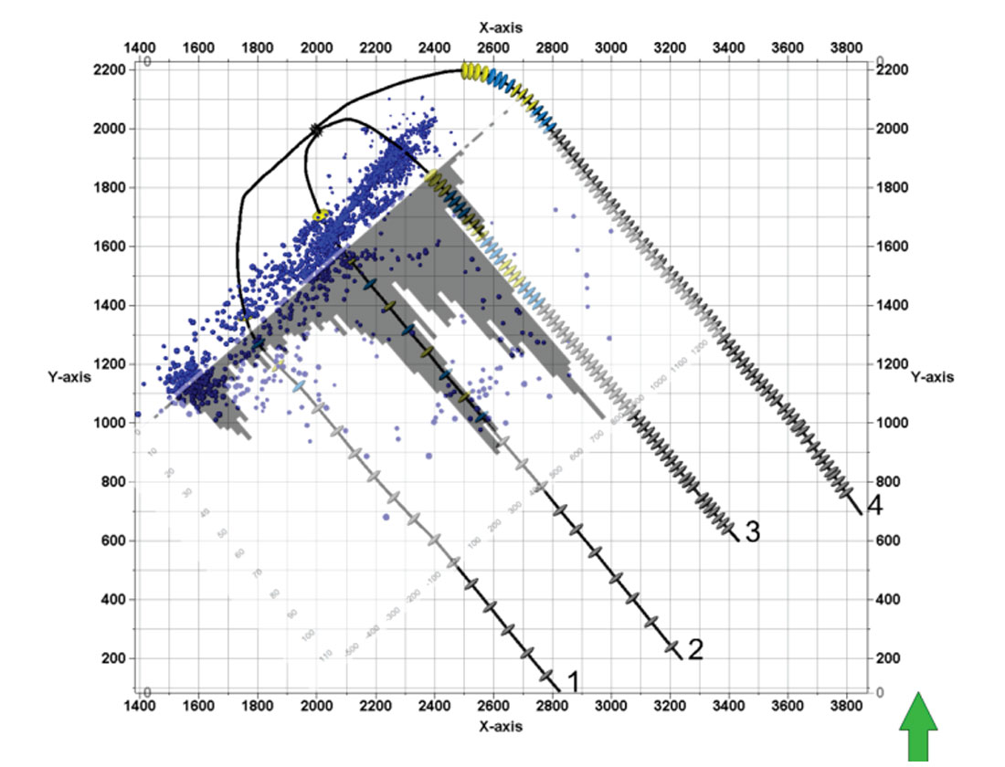
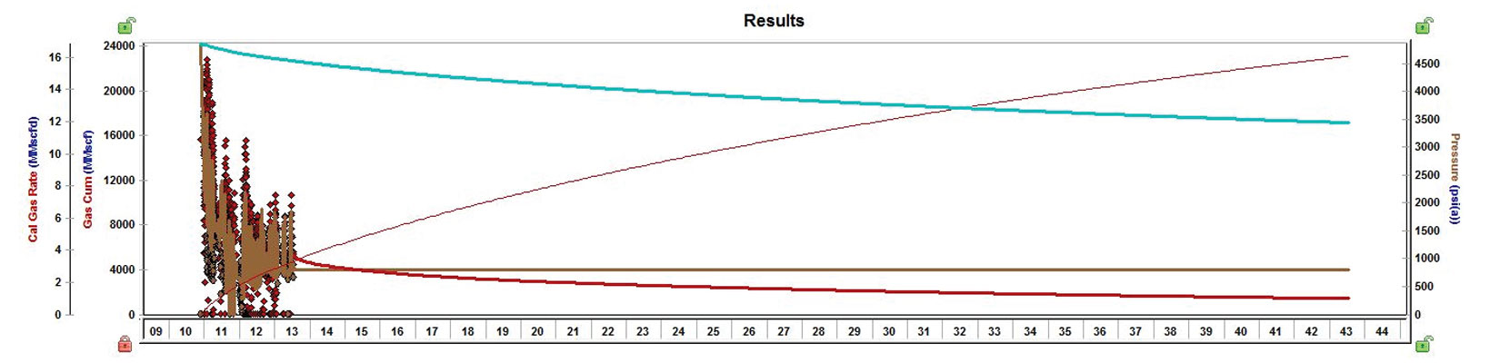
Figure 6a shows the analytical model schematic for Well 4. Figure 6b shows historical gas rate and bottom-hole pressure results of well 4 from the match. It is noticeable how much data was filtered, to be able to reduce average error on the history match process. Figure 6c shows the forecast of production of well 4 with an assumed bottom-hole pressure constrain, normally related to surface facilities constrains.
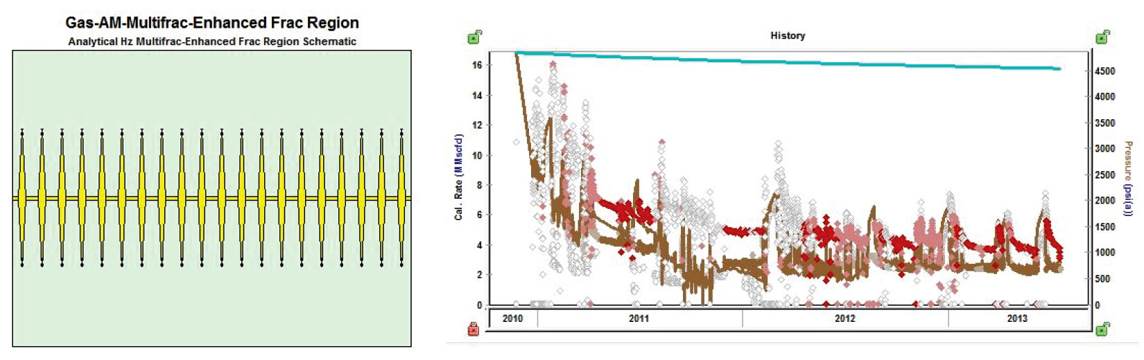
Figure 6b (right). History match of bhp of Well 4 showing synthetic reservoir pressure and gas rate.
Microseismic-derived Xf – Probabilistic approach
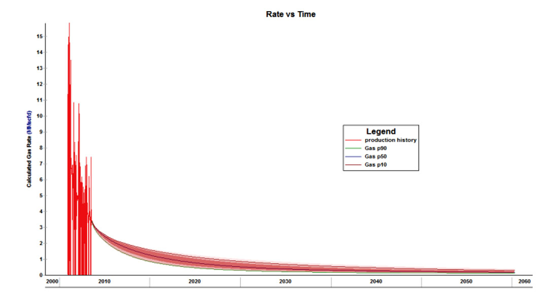
Figure 7a displays the Rate-Time probabilistic forecasts for Well 1. The calculated P90/P50/P10 forecasts are displayed overtop of the 99% confidence interval shading. The calculated P90/P50/ P10 forecasts are displayed overtop of the 99% confidence interval shading in Figure 7b.
Conclusions
- A workflow is described for a comparative interpretation of MS images in terms of Discrete Fracture Network geometry
- Comparing MS results could enable optimization of hydraulic stimulation by comparing the resultant geometry associated with alternate completion designs
- The resulting comparative MS interpretation can be used as part of a comparative hydraulic fracture evaluation to test the response to different designs and ultimately optimize the stimulation.
- Consistent and repeatable estimation of EUR from shale gas fractured reservoirs is problematic due to long-term transient effects and multifaceted well/reservoir geometry.
- A probabilistic approach to rate transient analysis and reserves evaluation is convenient because it empowers the investigation of many possible solutions. This also helps to address the non-uniqueness of analytical models.
- Building on previous work, the analytical enhanced fractured region model is used to create probabilistic production forecasts as follows:
- Randomly sampled SRV configurations and petrophysical inputs (km, Sg, porosity and hf) using Monte Carlo simulation.
- Regression techniques to define values for kSRV and FCD that optimally satisfy the history match.
- Forecast production for each run by means of fixed constraints on flowing pressure and terminal production rate.
- Microseismic-derived fracture half-length (xf) as an input.
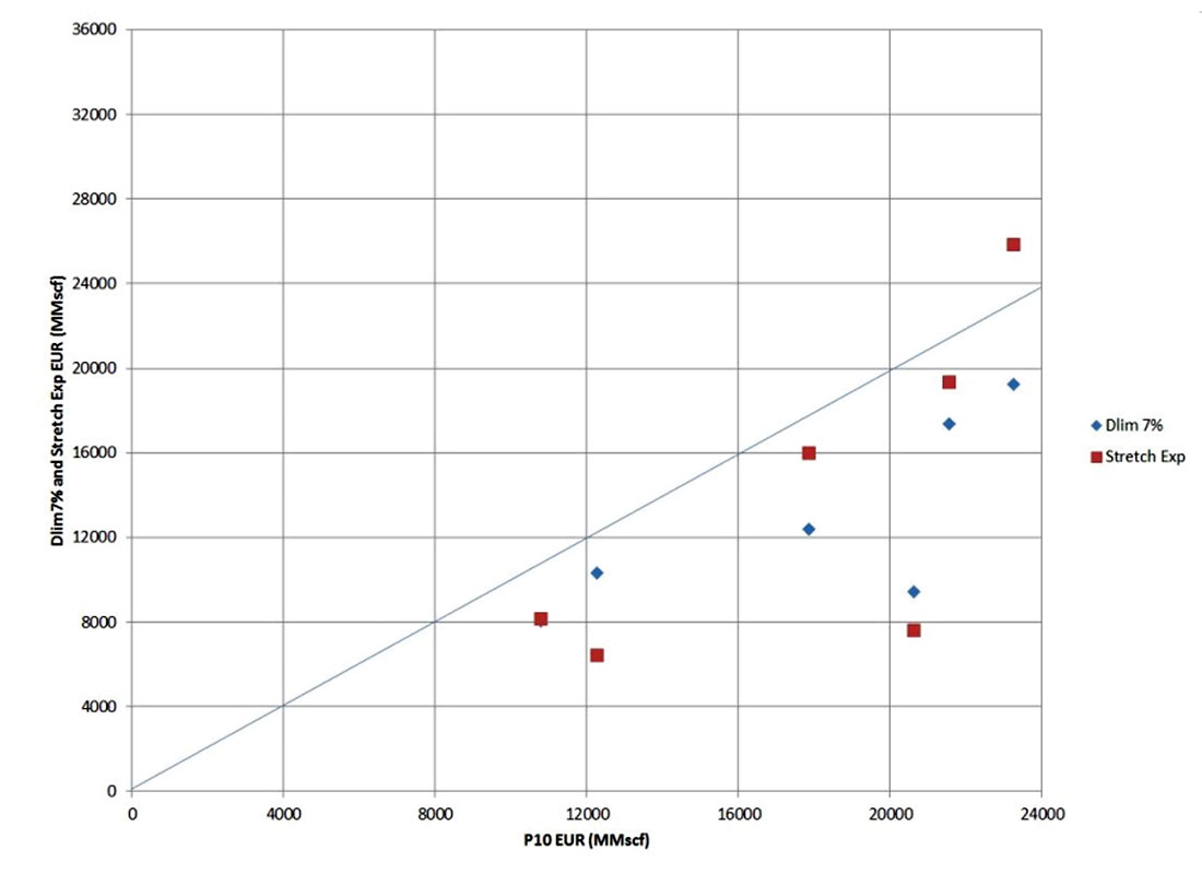
- Probabilistic forecasts compare well to stretched exponential and modified hyperbolic decline curve analysis, and help us remove outliers generated from these deterministic methods.
- The presented approach can easily be extended to include additional inputs of the selected enhanced fractured region flow model (such as stage spacing and initial pressure) or to other complex reservoir models. This approach can be applied to wells without production history as well, by simply removing the regression analysis and allowing the simulation to run unconstrained.
- The results from this case study indicate that the forecasts from the Enhanced Fractured Region model give a more optimistic forecast than deterministic case, however P10 forecast estimate is considered to be the upper bound for Proved + Probable + Possible. It is judicious to assume the rock surrounding the enhanced fractured region will contribute to long term production, but the extent of this contribution depends on the distance from the hydraulic fracture to permeability boundary xl, matrix permeability and the lateral length of the wellbore.
- The workflow described in this paper is defendable by physics and flow dynamics in the reservoir. Unlike empirical techniques, this workflow encourages the use of acquired information (flowing pressures, microseismic, PVT in case of liquid rich shale, etc) in order to obtain the best estimate of recovery.
- Production and microseismic data can be combined for forecasting production and estimating reserves.
- Statistically (combined with the use of analytics) the microseismic events can be analyzed and similarities among all stages distribution curves quantified.
- Further work is necessary to determine sufficient sample sizes and separate the modes of both distributions in the bimodal cases.
Nomenclature
| Ad | = Drainage area, ft2 |
| Ax | = Fracture exposed area, ft2 |
| ASRV | = Area of Stimulated Reservoir Volume, ft2md0.5 |
| AVk | = Bulk linear flow parameter form specialized plot, ft2 |
| b’ | = y-intercept of linear low straight line in the square root of time plot, (psi2/cp)/MMscfd |
| FCD’ | = Apparent fracture conductivity, dimensionless |
| hf | = Fracture height, ft. |
| k | = Permeability, md |
| km | = Matrix permeability outside stimulated reservoir volume, md |
| kSRV | = Permeability within stimulated reservoir volume, md |
| Le | = Horizontal well length, ft. |
| nf | = Number of fracture stages, dimensionless |
| rw | = Wellbore radius, ft. |
| T | = Reservoir Temperature, °R |
| tp | = Current production time, day |
| xl | = Distance from hydraulic fracture to permeability boundary, ft. |
| xf | = Half fracture length, ft. |
| Ye | = Distance between wells, ft. |

Acknowledgements
The authors would like to thank James Pyecroft and Doug Bearinger for the review of the manuscript prior submission.


Join the Conversation
Interested in starting, or contributing to a conversation about an article or issue of the RECORDER? Join our CSEG LinkedIn Group.
Share This Article