Wavelet estimation by non-linear optimization of all-pass operators

Abstract

A mixed phase wavelet can be parameterized as a convolution of a minimum phase wavelet and an all-pass wavelet. The minimum phase wavelet can be estimated from the data by the Wiener-Levinson algorithm. The technique of cumulant matching is used to estimate the phase of the all-pass wavelet. Higher order statistical methods, such as the cumulant matching deconvolution, are dependent on the bandwidth to central frequency ratio of the data. For the cumulants to be sensitive to the phase signatures, it is imperative that the ratio of bandwidth to central frequency is at least greater than one, and more favorably close to two. Pre-whitening of the data with the estimated minimum phase wavelet helps increase the bandwidth resulting in a more favorable bandwidth to central frequency ratio. The proposed technique makes use of this property to estimate the all-pass wavelet from the pre- whitened data. The paper also compares the results obtained from both pre-whitened and non-whitened data. The results show that the use of pre-whitened data results in a significant improvement in the estimation of the mixed phase wavelet when the data are severely band limited.

Introduction

Wavelet estimation is an important technique required to deconvolve the seismic data so as to obtain an estimation of the underlying reflectivity series. A reflection event is a spike which exhibits full band zero-phase signature. Convolution of the reflectivity with the source wavelet makes the reflectivity event lose its zero-phase and full band amplitude signature. Instead, it picks up the amplitude and phase signatures of the source wavelet. Deconvolution, with the assumption that the wavelet is minimum phase, removes the wavelet amplitude signature quite effectively. However, it leaves behind a spurious phase signature in the data. In order that the wavelet phase response is also effectively removed, it is necessary to deconvolve the data with an optimum mixed phase wavelet. Classical approaches such as Wiener-Levinson predictive deconvolution (Robinson and Treitel, 1980, Robinson, 1967, Peacock and Treitel, 1969) are intended to estimate the minimum phase wavelet in the data. These methods are based on second order statistical assumptions. It is well known that the second order statistical methods do not preserve the phase signature. Hence, there is a need to look for higher order statistical methods. Cumulants, which involve higher order statistical calculations, are known to preserve the amplitude and phase signatures of the wavelet. Unlike the third order cumulants, the fourth order cumulants do not vanish when the reflectivity series is symmetric (Walden and Hosken, 1986).

Many approaches were made to bypass the minimum phase assumption and estimate the wavelet that shows mixed phase character. Such methods include homomorphic deconvolution (Oppenheim et al, 1968; Ulrych, 1971, Ulrych et al, 1995), minimum entropy deconvolution (Wiggins, 1978), 4th order cumulants matching (Lazear, 1993), and others.

Tugnait (1987) proposed a fourth-order cumulant matching technique to estimate a mixed-phase moving average wavelet. Lazear (1993) applied this technique to the real seismic data. Velis and Ulrych (1996) applied the technique with a non-linear optimization approach. They estimated the mixed-phase wavelet from the fourth-order cumulant of the trace by means of Very Fast Simulated Annealing (VFSA) optimization method. They showed the dependence of the cumulant matching technique on the ratio of bandwidth to central frequency of the data.

An improvement over the previous cumulant matching approaches to mixed phase deconvolution is proposed here. The proposed technique does not involve root finding algorithm and does not need to solve large extended Yule- Walker system of equations (Porsani and Ursin, 1998; Porsani and Ursin, 2000). Parameterization of the mixed-phase wavelet as a convolution of a minimum phase wavelet with an all-pass wavelet can significantly simplify the problem. Deconvolving the seismic trace by the estimated minimum phase wavelet helps in broadening the bandwidth of the deconvolved data. This is a desirable effect. As pointed out earlier by Velis and Ulrych (1996) that a proper estimation of the mixed-phase wavelet by cumulant matching technique is possible when the ratio of the bandwidth to central frequency is greater than 1 and preferably close to 2. Hence, deconvolution by the estimated minimum-phase wavelet works favorably for the cumulant matching technique. Optimization for the all-pass wavelet is performed by means of VFSA technique (Sen and Stoffa, 1995, Velis and Ulrych, 1996).

Development of The Algorithm

With the assumptions that the reflectivity series is non- Gaussian, stationary and a statistically independent random process, the fourth order cumulant of the trace is equal to, within a scale factor, the fourth order moment of the wavelet. Cumulants and moments are defined in the appendix. With the same analogy, it can be said that, when the wavelet is parameterized as a convolution of a minimum phase wavelet and an all-pass wavelet, the fourth-order cumulant of the whitened trace (deconvolved by the minimum phase wavelet) is equal to, within a scale factor, the fourth-order moment of the all-pass wavelet. The minimum phase wavelet estimated from the autocorrelation of the trace has the same amplitude spectrum as that of the true mixed phase wavelet. Thus, deconvolving the trace with the minimum phase wavelet not only removes the wavelet amplitude spectrum from the data but also increases the bandwidth. This is a favorable result as a higher ratio of the data bandwidth to central frequency is desired for the wavelet estimation. The whitened trace now contains only the phase information of the wavelet. Hence, an all pass wavelet remains to be optimized from the whitened data.

where d_t is the seismic data, r_t is the reflectivity series and p_t is the mixed phase wavelet. The ‘*’ indicates the convolution process. As mentioned earlier, pt can be parameterized as the convolution of the minimum phase wavelet and the all pass wavelet (Porsani and Ursin, 1998). Thus,

where p̃_t is the minimum-phase wavelet estimated from the trace and f_t is the all-pass wavelet. The Z-transform of the all-pass wavelet can be written as (Porsani and Ursin, 1998)

with B(Z)=b₀+ b₁Z+ b₂Z² +...+ b_aZ^a and the term Z^a accounts for the time shift required to make the all-pass wavelet causal. It is important to mention here that the time series b_t= b₀,b₁, . . . ,b_a is minimum phase. This is a very simple parameterization with b_t=b₀, b₁, . . . ,b_a as unknowns. For this problem, the term Z^a in the equation (3), is not important because it only accounts for the time shift in the final estimator of the wavelet.

Substituting for p_t in equation (1),

In the Z- domain,

Deconvolution by the minimum phase wavelet yields

where, D_w(Z) is the deconvolved trace that has been whitened by the removal of the minimum phase wavelet. Thus, the reflectivity sequence can be obtained by deconvolving the whitened trace by an optimum all-pass wavelet.

Taking the Z-transform of both sides of equation (2),

This can be further written as,

where |P(Z)| is the amplitude spectrum of the mixed-phase wavelet, |p̃(Z)|is the amplitude spectrum of the estimated minimum phase wavelet and |F(Z)| is the amplitude spectrum of the all-pass wavelet, which is equal to 1. Also, θ(Z) is the phase of the mixed phase wavelet, θ_min(Z) is the phase of the minimum phase wavelet, and θ_F(Z) is the phase of the all-pass wavelet.

Since |P(Z)| = |p̃(Z)|,

The problem of estimating the mixed-phase wavelet can now be posed as a problem of estimating the optimum phase of the allpass wavelet.

Testing the Algorithm

The proposed algorithm for estimating the mixed-phase wavelet is tested by designing a synthetic mixed phase wavelet and a synthetic trace. Table 1 shows the roots of the Z-transform of the wavelet coefficients that are considered to generate the synthetic mixed-phase wavelet.

Table 1. The roots of the synthetic wavelet. Negative phase angles indicate the complex conjugate of the corresponding roots.
No.	1	2	3	4	5	6	7	8	9
Magnitude	1/1.3	1/1.5	1/1.11	1.2	1.3	1.8	1.95	1.25	1.8
Phase (degree)	0	0	+45 -45	+5 -5	+60 -60	0	180	+120 -120	+160 -160

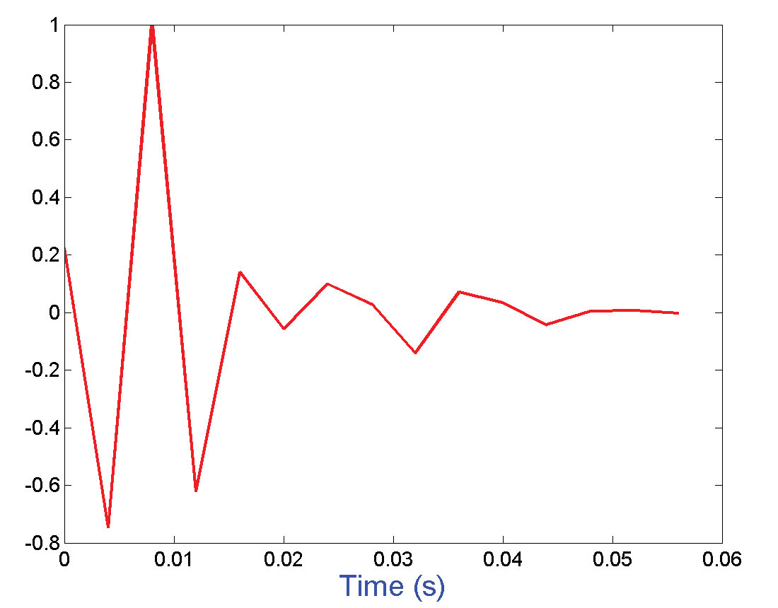
Figure (1) shows the true synthetic wavelet. A synthetic trace was generated by convolving a Laplacian mixture distribution of reflectivity sequence (length N = 250) with the true mixed phase wavelet. The trace does not contain any noise component. Figure (2) shows the estimated minimum phase wavelet obtained from the data by the Wiener-Levinson algorithm. The whitened trace was obtained by deconvolving the data by the estimated minimum phase wavelet. The whitened data contains only the phase information of the wavelet, as the amplitude information has been effectively removed by the deconvolution. Hence, the technique of cumulant matching reduces to the matching of the fourth-order moment of the all-pass wavelet and the fourth-order cumulant of the whitened trace.

Fig. 01 — Figure 1. The true synthetic mixed phase wavelet.

Fig. 02 — Figure 2. The estimated minimum phase wavelet.

The phase estimation by cumulant matching technique is performed by using VFSA, a non-linear optimization tool. VFSA was used to optimize for the model parameters b_t = b₀, b₁,..., b₉ which form the denominator term of the all-pass wavelet (equation 3). The unknowns here are the length of b_t and its coefficients. The optimization is performed on varying lengths of b_t (minimum length is 2 with coefficients b₀ , b₁ and maximum length is 10 with coefficients b_t = b₀, b₁,..., b₉). This resulted in 9 numbers of estimated wavelets. As mentioned earlier, b_t= b₀, b₁,..., b_a is minimum phase. This a priori information was incorporated in the VFSA algorithm by multiplying the model parameters with a decay function given by Aⁿ, n = 0, 1, 2…,α. Where, A < 1 and α = length of the model parameters (Lazear, 1984). The cost function for the optimization is given by

Where,

is the fourth-order trace cumulant (normalized by the central lag cumulant) and

is the fourth-order wavelet moment (normalized by the central lag moment). An explanation on the cost function is provided in the appendix.

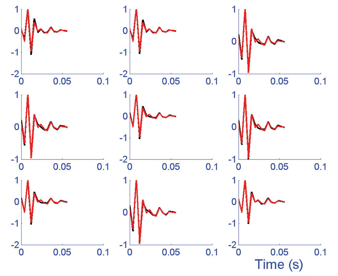
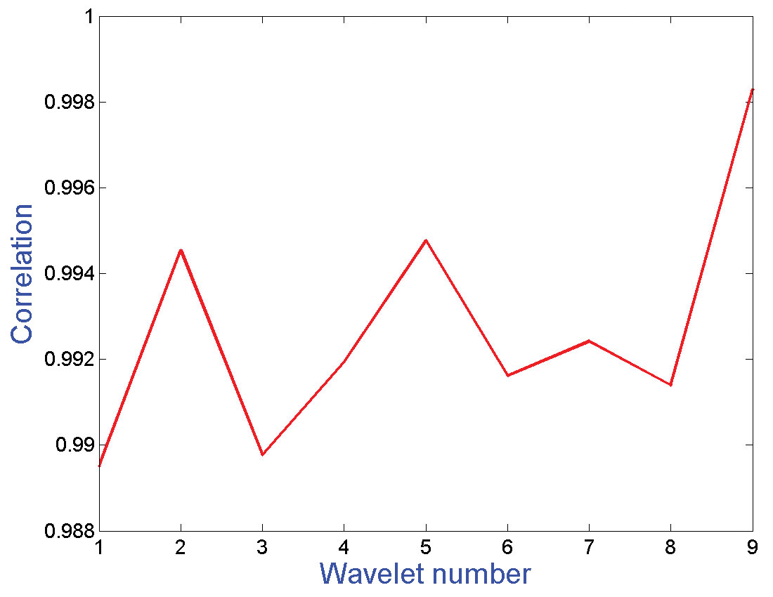
Fig. 03 — Figure 3. The estimated wavelets plotted on top of the true wavelet. Each of the wavelets corresponds to different lengths of the model parameters. For example, the plot on the top row left shows the estimated wavelet for *b_t = b*₀*, b*₁. The plot on the top row middle shows the estimated wavelet for *b_t = b*₀*, b*₁,b₂ and so on till the last plot (bottom row right) that shows the estimated wavelet for *b_t = b*₀*, b*₁*,..., b*₉. The length of the reflectivity series is N = 250.

Figure (3) shows the estimated wavelets plotted on the top of the true wavelet. As mentioned before, each estimated wavelet corresponds to different lengths of bt . It is observed that, for most of the estimations, the wavelet is reasonably well estimated. The correlation measures of the estimated wavelets are shown in the figure (4). The correlation measures are high for all the cases.

Fig. 04 — Figure 4. Correlation measures for the estimated wavelets. Wavelet number =1 corresponds to *b_t = b*₀*, b*₁. Wavelet number = 2 corresponds to *b_t = b*₀*, b*₁,b₂ and so on till wavelet number = 9 that corresponds to *b_t = b*₀*, b*₁*,..., b*₉.

Comparison of the Algorithm

A comparison is called for between the estimation of the mixed-phase wavelet with the proposed algorithm and that directly obtained from the data. The cumulant matching technique is not sensitive when the data bandwidth to central frequency ratio is less than 1. Hence, it is expected that cumulant matching technique will not be able to perform well when the mixed phase wavelet is estimated from severely band limited data having the ratio of bandwidth to central frequency less than 1. The proposed technique has the advantage of removing the wavelet amplitude spectrum from the data, thus resulting in a wider bandwidth of the whitened data. This allows the cumulant matching technique to work in a favorable domain and hence the result is expected to be better.

Fig. 05 — Figure 5. The true band limited mixed phase wavelet (left). The estimated minimum phase wavelet (right).

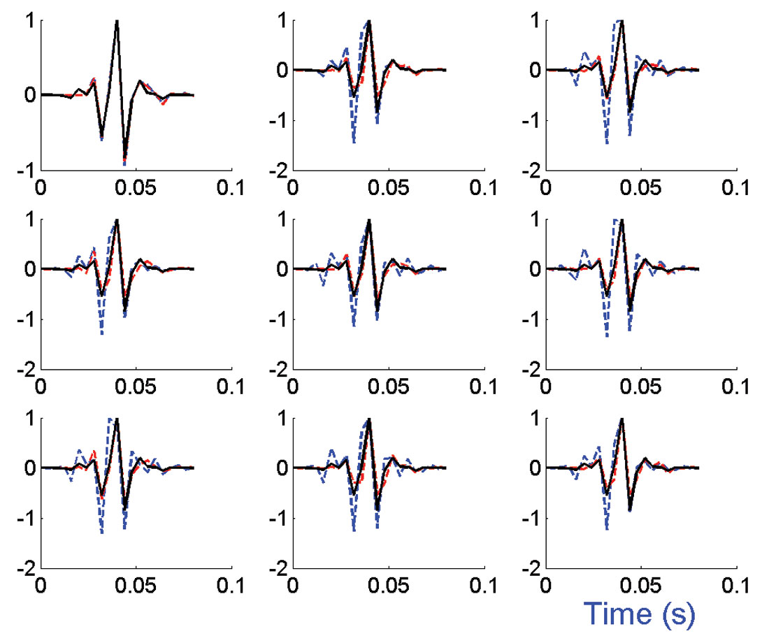
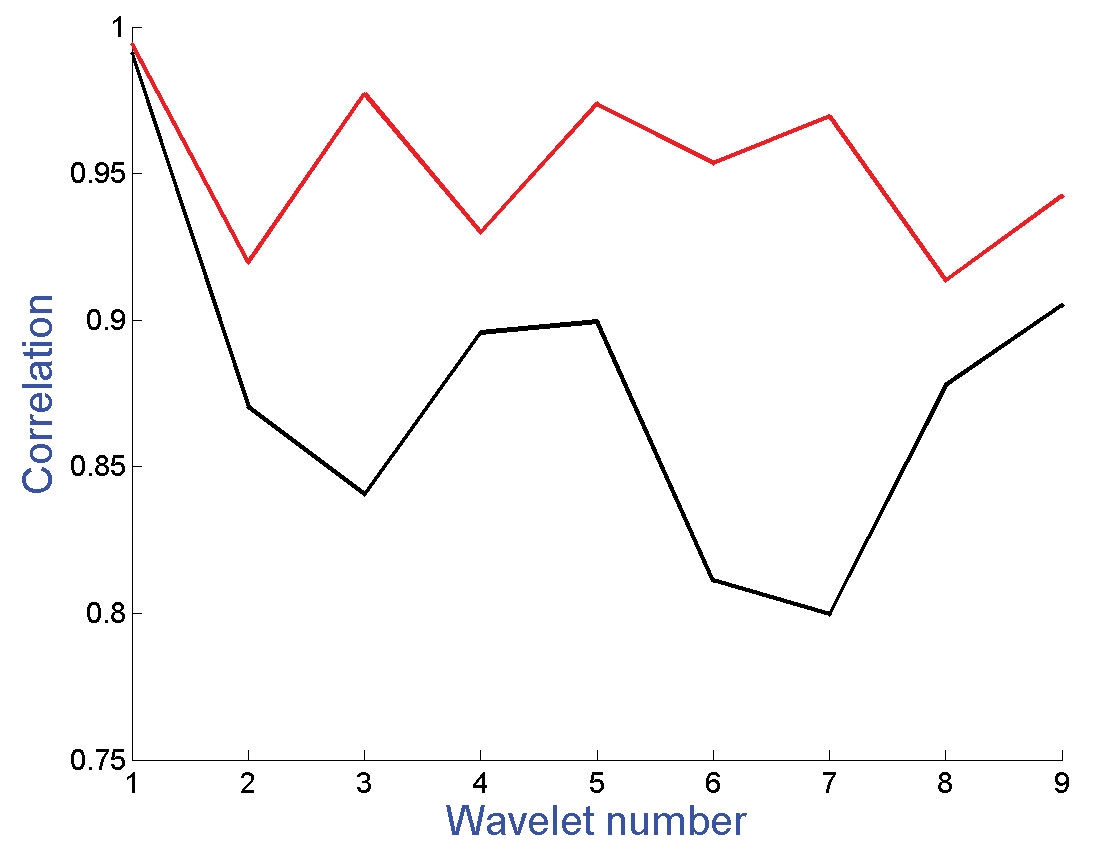
A mixed phase wavelet with a bandwidth to central frequency ratio of 0.5 is chosen for the purpose of illustration here. Figure (5) shows the true band limited wavelet and the corresponding minimum phase wavelet estimated from the data. A synthetic trace was generated by convolving the true mixed phase wavelet with a reflectivity sequence of length N equals to 250. The underlying reflectivity sequence was Laplacian mixture in distribution. The synthetic trace thus generated was whitened by deconvolving with the estimated minimum phase wavelet. Figure (6) shows the estimated wavelets plotted on the top of the true wavelet for a given set of model parameters bt . As before, the optimization by VFSA was performed on 9 different lengths of b_t (minimum length was 2 with coefficients b₀,b₁ and maximum length was 10 with coefficients b_t = b₀, b₁,..., b₉). The red line shows the estimated wavelet obtained from the whitened trace and the blue line shows the estimated wavelet obtained from the actual (non-whitened) trace. The black line shows the true wavelet. The estimated wavelets obtained from the whitened data correlate much better than those of the estimated wavelets obtained from the non-whitened data. This observation corroborates the fact that the cumulant matching technique is sensitive to the ratio of the bandwidth to central frequency. A better estimation of the wavelet was obtained because this ratio could be improved by whitening the trace with the minimum phase wavelet. Figure (7) shows the correlation measure plotted for the individual estimated wavelets. It is observed that the estimation from the whitened data has greater correlation for all the wavelets as compared to the wavelets estimated from the non-whitened data.

Fig. 06 — Figure 6. The estimated wavelets plotted on top of the true wavelet. The red line represents the wavelets estimated from the whitened data. The blue line represents the wavelets estimated from the non-whitened data. The black line represents the true mixed phase wavelet. The plot on the top row left shows the estimated wavelets for *b_t = b*₀*, b*₁. The plot on the top row middle shows the estimated wavelets for *b_t = b*₀*, b*₁, b₂ and so on till the last plot (the bottom row right) that shows the estimated wavelets for *b_t = b*₀*, b*₁*,..., b*₉. The length of the reflectivity series is N = 250.

Fig. 07 — Figure 7. The correlation measure for the estimated wavelets for each set of model parameters. Correlation is compared between the wavelet correlation obtained from the whitened trace and that obtained from the non-whitened trace. The black line is the correlation for the wavelets estimated from the non-whitened trace. The red line is the correlation for the wavelets estimated from the whitened trace. The comparison shows that the correlation is higher when the wavelets are estimated from the whitened trace. Wavelet number = 1 corresponds to *b_t = b*₀*, b*₁. Wavelet number = 2 corresponds to *b_t = b*₀*, b*₁, b₂ and so on till wavelet number = 9 that corresponds to *b_t = b*₀*, b*₁*,..., b*₉.

Conclusions

Cumulant matching technique works well when the bandwidth to central frequency ratio in the data is greater than 1. The technique is best suitable when this ratio is close to 2, i.e. the data is full band. The proposed technique separates the minimum phase part of the wavelet from the data by deconvolving the data with an estimated minimum phase wavelet. As a result, the deconvolved data contains only the phase signature of the mixed-phase wavelet. This also allows the cumulant matching technique to work in a favorable regime of the bandwidth to central frequency ratio. The synthetic examples showed that very fast simulated annealing can be used quite effectively to estimate the all-pass wavelet and hence the mixed phase wavelet. The paper also presented a comparison when the wavelet is estimated from the whitened data and non-whitened data. The proposed algorithm allows for whitening the data using the estimated minimum phase wavelet. It is observed that when the data were severely band limited, the estimated mixed phase wavelet, in general, had relatively poor correlation with the true wavelet. However, suitable parameterization of the wavelet, and subsequent whitening of the data, improved the estimation of the mixed phase wavelet. The plot of the correlation measure for the estimated wavelets obtained from the whitened data shows higher correlation value as compared to those wavelets obtained from the non-whitened data. This is an encouraging result for the proposed algorithm.

End

Acknowledgements

We would like to acknowledge to Drs. Neil D. Hargreaves, Milton Porsani and Danilo R. Velis for sharing their valuable thoughts on wavelet estimation.