Don’t ignore seismic attenuation

In general terms, seismic attenuation is the loss of elastic energy contained in a seismic wave, occurring through either anelastic or elastic behaviour. Anelastic loss, or intrinsic attenuation, is a result of the properties of the propagation medium. It causes a fraction of the wave’s energy to be converted into other forms such as heat or fluid motion. Non-intrinsic effects like multiple scattering are collected under the term apparent attenuation; they are so many and varied that intrinsic attenuation is difficult to isolate.

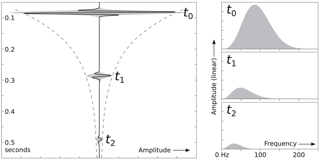
Attenuation of a seismic wave results in amplitude loss, phase shifts due to the associated dispersion, and the loss of resolution over time. This makes interpretation of the stacked data more difficult, and introduces an amplitude gradient in pre-stack data that is not predicted by reflectivity alone. These problems can be mitigated by the use of an inverse Q-filter which attempts to reverse the attenuation effects based on a measured attenuation field. Measures of attenuation are useful in their own right, because through them we can infer reservoir properties for characterization purposes.

The mechanisms of intrinsic attenuation have been referred to as either jostling or sloshing losses, relating to losses from dryframe or fluid-solid interactions respectively. Jostling effects involve the deformation or relative movement of the rock matrix, for example due to friction from intergranular motion or the relative motion of crack faces. More significant in magnitude are the sloshing effects, which occur when pore fluids move relative to the rock frame. These fluid effects are characterized by the scale over which pressure is equalized, from large-scale Biot flow, between the rock frame and the fluid, to squirt flow caused by the compression of cracks and pores.

Attenuation may be described as the exponential decay of a seismic wave from an initial amplitude A₀ to an attenuated state A over distance z, quantified by an attenuation coefficient α:

A = A₀ e^-αz

Various models describe the behaviour of α with frequency, and the relationship between the frequency- dependent velocity V(f) and the quality factor Q. Although many of the intrinsic attenuation mechanisms, specifically the sloshing losses, are dependent on frequency, Q is often assumed to be constant over the limited bandwidth of seismic experiments, resulting in α being linear with respect to frequency: α = rf VQ.

Q may also be defined by the complex behaviour of the elastic modulus M:

Q = Re (M) Im (M)

Seismic attenuation may be measured from different experimental configurations and at different frequency scales. The general method is to analyse the change in amplitude or frequency content or both, with propagation distance. For exploration seismic, two of the more common approaches are:

1. Spectral ratio – The spectrum is observed at two points along its travel-path, S₁(f) and S₂(f), with a time separation Δt. There is an inverse linear relationship between Q and the natural logarithm of the ratio of S₂ to S₁:

The intercept term is determined by frequency independent amplitude effects such as energy partitioning P and geometric spreading G.

2. Frequency shift – In which the shift of the centre frequency of the spectrum is related to attenuation of a modelled spectrum.

Seismic attenuation is rarely estimated – it is an often overlooked attribute. But the desire for quantitative geophysical attributes and improved data quality should win it more attention, especially as high-fidelity data allow ever more quantitative analysis. The effects of attenuation can no longer be ignored.

 

Q & A

The title of your short article is ‘Don’t ignore seismic attenuation’. I think it is a good title. You mention two methods for determination of attenuation, namely the spectral ratio method, and the frequencyshift method. Which of the two methods is (a) easier to use, (b) more accurate, and (c) more widely used?

Let me first very briefly introduce the two methods before I comment on them individually. In the spectral ratio method, the natural logarithm is taken of the ratio between an attenuated and initial spectrum. For an exponential-decay with a constant Q, this becomes a linear function with respect to frequency (as well as time delay). A representative bandwidth is chosen, and the slope of the linear relationship is inverted, yielding a Q value. The frequency-shift method assumes a wavelet spectrum of a known model (e.g. Gaussian) that can be described by a single parameter, namely the centroid frequency (other methods exist using the dominant frequency). Attenuation causes the centroid frequency to shift, which can be described analytically from the equation of the spectral model. Therefore, by knowing the shift in frequency, Q can be calculated.

In my experience, the spectral-ratio method is more widely used than frequency-shift methods. As for ease of use, I would say that both are simple procedures to perform, however the spectral-ratio method is perhaps more intuitive. The accuracy part of the question however, is perhaps less obvious.

Accuracy is a difficult claim to make. There are many comparisons of methods, published or not, that fall into two categories: 1) simple synthetic models and 2) real data examples. In the first type, the attenuation is known, and the results show which method has better mathematical accuracy. Occasionally random noise is added in, which allows a determination of the methods’ robustness to simple noise. Accuracy claims made on this type of test don’t particularly hold much weight in my opinion, beyond demonstrating a proof of concept. The second type of test is obviously more realistic but suffers the problem of not knowing what the true attenuation is. Therefore, secondary information is required to help suggest which method is more accurate, which is also not a very conclusive argument. What really needs to be done is to compare methods using realistic synthetic data that incorporate thin-bed effects and non-white reflectivity in order to introduce realistic spectral interference to the data. I think what you would find is that one method is not simply better, but likely just better in certain situations.

Errors in both methods tend to stem from the fact that spectra are not always well behaved. Often, the spectra are significantly notched, and notched differently at the reference and measured locations. For the frequency-shift method, this can have a large impact on the calculation of the centroid frequency, which is the sole parameter of the method. For spectral-ratios, this can cause non-linear behaviour, which can be exacerbated by a poor choice of inversion bandwidth.

My preference is for the spectral-ratio method because of its flexibility. First of all, the spectral-ratio method also allows for any range of inversion techniques to help make the process more robust. These include appropriately weighting the points in the spectrum to reduce the influence of noise and even inverting multiple time separations simultaneously to combat the effects of spectral notching. There is also no need for Q to be constant in the spectral-ratio method, as other functions can also be inverted.

Attenuation correction in terms of inverse Q filtering has been around for over 40 years. Why do you think we have not been able to make significant headway in the determination of accurate Q values and their application to seismic attenuation?

This is a good place to say that I think there are two levels of attenuation that we can measure, which is in many ways analogous to velocity. With velocities for instance, there are processing velocities that optimally flatten the gathers and there are velocities that are suitable for reservoir characterization, for example from a VSP or full-waveform inversion. Just as detailed velocities would not necessarily flatten gathers, NMO velocities are insufficient to estimate reservoir properties. The same is true with attenuation. Recovering high frequencies and applying dispersion corrections is not terribly sensitive to the choice of Q. For these purposes, coarse estimates of Q over longer time intervals are sufficient. However, this Q is not going to be useful for reservoir characterization. Detailed Q-estimates for reservoir characterization should be done on prestack data with a robust methodology to reduce thin-bed effects and processing artifacts, including those from stacking.

So why is it rare to see detailed Q measurements in practice? I think it’s primarily because geophysicists restrict their understanding of attenuation to something that can improve resolution and phase. Why go to the effort of detailed analysis of your data, when a coarse Q measurement would be sufficient? Indeed, even simple time-variant spectral whitening is a type of blind Q-compensation and that requires no effort of estimating Q. I think accurate Q values suitable for reservoir characterization will become more mainstream once people start to see the benefits of Q beyond resolution and phase improvements.

You rightly mention that attenuation of a seismic wave results in amplitude loss, phase shift and loss of resolution. If the attenuation correction we apply using either of the two methods is not accurate, it would result in incomplete amplitude, phase or frequency compensation. Do you think that is a good practice? Alternatively, do you think we can determine the Q values for application in an accurate way?

This is very much linked to what I mentioned in the previous question about having different levels of Q estimation, and in this case I think we are talking about the coarse level of estimation. Of course I would never think that it is ideal to have an incomplete compensation of the properties that you mention, but I think it is worth having a look at the alternative which is often standard practice.

Much of our seismic data is processed with an application of spectral whitening or spectral balancing. Every company has their own way of doing this, but the general goal is to achieve a flat spectrum. If this is not done in a time-variant manner, the process is non-physical, and the shallow data are being enhanced artificially relative to the deeper data. If it is time variant, there is not any thought put into what Q would be required to justify that correction. Dispersion corrections are almost never applied in my experience.

I think this shows we have become accustomed to accepting frequency enhancement without thinking about the physical meaning. Therefore, I would say that even using an imperfect Q for an inverse filter is doing better than a process that doesn’t try to incorporate a realistic value. As for dispersion, Duren and Trantham (1997) demonstrated that Q does not have to be estimated accurately to remove the majority of dispersion and reduce the phase error.

Again as you mention, measures of attenuation can be used to infer reservoir properties. How much of this is being done in our industry and if not what is preventing us from using it effectively?

From my experience I would say that very little is being done with Q for estimating reservoir properties. Occasionally there are articles that show a qualitative interpretation of a Q map (however accurately or coarsely it is estimated) as being “due to gas”. However there has been some excellent research that shows the utility of attenuation for more quantitative purposes, for example Q_S:Q_P ratios or 4D attenuation to determine more accurately the variations in gas saturation.

I think one of the barriers for many geophysicists is that to make these quantitative interpretations, an appropriate rock-physics model is needed. In fact, these exist in abundance, but choosing the appropriate model for the situation at hand, defining the assumptions in the models, and simply trying to understand or implement them can be quite daunting, even for geophysicists that are familiar with their existence. The other barrier of course is how to make these detailed measurements, and while methods have been published (Reine et al., 2012a,b) they are by no means common.

What do you think could be done to bring more attention to the determination of attenuation correction to seismic data?

I will unfairly put the spotlight on the service companies for this one. I say that because much of the knowledge and opinion of what should be done to seismic data in processing comes from what the service companies recommend in meetings and present at technical talks. I recognize, of course, that in order for this to be a priority for them, there has to be a demand from the industry, so it is a circular argument.

Strictly speaking on attenuation corrections, a useful and convincing case study would show how Q was determined, how the inverse filter was applied, and why that is better than a) nothing, b) spectral whitening, and c) time-variant spectral whitening, highlighting the benefits of not only resolution, but phase correction as well. Few service companies talk about Q compensation and the comparisons tend to be with compensation versus with nothing. This obviously makes the Q compensation look good, but does nothing to convince geophysicists that it is better than other frequency-enhancement processes.

Apart from the accuracy of the compensated signal through inverse Q filtering, the numerical instability in the estimation of the exponential functions is a problem that leads to artifacts and increases the background noise. This has led to discouragement in the use of Q compensation. If we don’t correct for the attenuation, it could lead to poor seismic interpretability and contribute to seismic-well data misties. Could you comment on this?

The exponential-decay nature of attenuation would seemingly be easily corrected by an exponential gain. In the noise-free case with perfect instrument fidelity, this would be true, but as you point out, noise tends to run away on us. The inverse-Q filter detailed by Wang (2002) is stabilized to act only on the seismic bandwidth not dominated by noise. Also, van der Baan (2012) has shown that inverse Q filtering is ideally suited for dispersion corrections (the phase component), and the spectral amplitudes are better compensated for using a timevarying deconvolution, which similarly acts only in the wavelet pass band thereby limiting background noise.

I lean towards accepting more noise for the added advantages of increased resolution, but of course like all processing, this should be driven by the data. If the data are inherently noisy, then maybe the lack of resolution isn’t the biggest problem. There’s no point making the data unusable for the sake of being theoretically correct. Conversely, if a geophysicist is going to do some sort of resolution enhancement, why not use one that has a more sound theoretical standing, correcting for spectral amplitude and dispersion with a measured Q, rather than an arbitrary spectral gain with no phase component. It is worth pointing out that spectral whitening also increases the noise content in data. Start asking about inverse-Q filters from your processor, and sound Q compensation will move up in the priorities.

References

Duren, R.E., and E.C. Trantham, 1997, Sensitivity of the Dispersion Correction to Q Error: Geophysics, 62, 288-290.

Reine, C., R. Clark, M. van der Baan, 2012, Robust Prestack Q-Determination Using Surface Seismic Data: Part 1 – Method and Synthetic Examples: Geophysics, 77, R45-R56.

Reine, C., R. Clark, M. van der Baan, 2012, Robust Prestack Q-Determination Using Surface Seismic Data: Part 2 – 3D Case Study: Geophysics, 77, B1-B10.

van der Baan, M., 2012, Bandwidth Enhancement: Inverse Q filtering or Time-Varying Wiener Deconvolution?: Geophysics, 77, V133-V142.

Wang, Y., 2002, A Stable and Efficient Approach of Inverse Q Filtering: Geophysics, 67, 657-663.