6D Interpolation of Seismic Data – Rationale, Practice and FAQs

For many reasons, such as acquisition limitations, economic constraints, and merging data of various shooting parameters from different vintages, seismic data needs to be regularized, upsampled, reconstructed and interpolated. Furthermore, a common deliverable of interpolation is regularized prestack data which will improve many state-ofthe- art inversion processes and migration imaging.

In recent years, better and more accurate interpolation algorithms have been developed. To name a few major examples, there are:

• Prediction filters (Spitz, 1991; and Wang, 2007)
• Rank reduction method (Trickett et al., 2010; and Naghizadeh, 2013)
• Minimum weighted norm interpolation, MWNI method (Liu et al., 2004)

There is a long list of methods described by Stanton and Sacchi (2013). Of many elegant methods, 5D MWNI (Trad, 2009 and 2014) is probably the most popular method among them because it more closely maintains the original input trace characteristics including signal-tonoise ratio than the other methods.

Data scenarios that challenge most interpolation methods include:

• Data with random missing traces. This is considered the least evil kind of data scenario for interpolation because it boils down to a de-noising exercise for interpolators.
• Data with a gap of missing traces. Depending on the size of the gap, this data can be very difficult to interpolate.
• Data which has aliasing in space. This happens when structural data is not adequately sampled and recorded in space.
• Data with curving events or diffractions. This violates many interpolators that rely on the plane wave or bandlimited sparsity assumptions unless the data is subdivided into smaller blocks to make the curving events locally linear.
• Data with regularly missing traces. This may be considered as upsampling of spatial data. An example of this is the popular Mega-Bin acquisition. It is the most challenging of interpolations especially when the data is structural and the steeper dips are aliased.

We will demonstrate how our new 6D interpolation stands up to these challenges.

The motivations for 6D Interpolation

The industry standard 5D minimum weighted norm interpolation (MWNI) starts data fitting from the stable low frequency slices, one slice at a time, and recursively layer-by-layer works its way up to higher frequencies. There is no global data insight extracted from the frequency- wavenumber domain since an independent 4D MWNI is applied in space for every frequency slice, one slice at a time. This unconstrained fitting can lead to inaccurate results under challenging scenarios such as meager data support, upsampling of regularly missing data, or aliased dips. Curry (2010) and Naghizadeh (2012) suggested imposing a Fourier-radial thresholding mask during data fitting, a method that is not MWNI based, and such a strong constraint could lead to results that are somewhat too smooth.

Ng and Negut (2013, 2014) integrated the Fourier-radial angular weight (Aw) concept into MWNI, thereby raising the dimension of the MWNI by one. As a natural extension to 5D interpolation, Ng and Negut (2015, 2016a) proposed the 6D interpolation method which has an additional dimension along multi-angular directions which is added to the 5D MWNI to guide the a priori model in the frequency-wavenumber domain. The angular weights are derived from scanning the input data in the frequency-wavenumber domain along many radial directions pointing away from the origin which correspond to the data dips. Angular weights connect data information across all frequency-wavenumbers globally. This is crucial to accurate de-aliasing of data, and is missing in conventional 5D MWNI. A related method is that of Chiu (2013, 2014) which uses a model-constrained MWNI by dip scanning a few major dips in the time-space domain. This method essentially does two interpolations: first for the a priori model building, and then for the actual MWNI. 6D AwMWNI performs the angular weight ‘scan’ and the MWNI in the frequency-wavenumber domain in one step, giving a speed advantage.

There is a good analogy for 5D interpolation – the process of laying bricks when building a fire pit from low level to high level without using global plumb line reference. Even with a good foundation level to start with, this could eventually lead to an undesirable slanting brick structure at the top levels. But when a plumb line reference is used, which in our case is the angular weight function, or the sixth dimension, it guides the 5D MWNI engine, resulting in a stable 6D interpolation method, and meets the objective of preserving structural integrity of the data after interpolation (Ng and Negut, 2016b).

Methodology

Suppose d(x,y,h,g,f) is the complete 3D prestack data in 5D space: inline x, crossline y, offset x indicated by h, offset y indicated by g, and f frequency; and its corresponding 4D spatial Fourier transform is D(kx,ky,kh,kg, f).

At any frequency f, the desired unknown complete data can be written as

where F^H is the 4D wavenumber inverse, Fourier transform operator, D (i.e . |D| ) the unknown 4D complete data amplitude spectrum, m the unknown 4D ‘model’ phase, and H the conjugate transpose.

However, what is given is the observed incomplete data masked by the known sampling matrix T,

By forming the adjoint operator, the model phase

can be found through data fitting by the conjugate gradient method.

A reasonably close approximation of the complete amplitude spectrum D at each frequency slice as the a priori D₀ to initiate the inversion. The better the a priori, the better the inversion quality and the faster the conversion.

Conventional 5D MWNI simply uses the updated result estimated D from previous frequency f-1 as the a priori of current frequency f,

Since the spectral information at f-1 has no foreknowledge of the information at the next higher frequency f, such a priori is biased towards the lagging frequencies without a global insight of the data. So, under previously mentioned challenging data scenarios, D can be inaccurately estimated and would then mislead the subsequent inversion.

In contrast, we use a multidimensional Fourier-radial angular weight gamma γ that conditions the known input unbiased incomplete data amplitude spectrum to get the a priori D₀ at any point in frequency, whilst not lagging behind in frequency:

where p is an arbitrary non-negative power controlling gamma γ sharpness. If either p = 0 or γ = 1, there is no angular weight or global data insight, and equation (5) degenerates to equation (4), the conventional form of 5D MWNI. The angular weight gamma γ has a uniform amplitude in the Fourier-radial direction and is defined as

where A is the normalized angular sum of amplitude spectral values along the Fourier-radial direction of all usable apparent dip angles, Θ_i,

This method adds one extra angular dimension to the conventional 5D MWNI by connecting spectral information across all frequency-wavenumbers, which is crucial to the de-aliasing of dipping data but missing from conventional 5D MWNI. In doing so, 5D MWNI becomes 6D AwMWNI. In practice, k_x and k_y of gamma γ in equation (6) describe the structure dips which are essential to 6D, while k_h and k_g of γ describe the data residual or linear move-out whose improvements are a diminishing return. Dropping the k_h, k_g terms improves speed.

Example 1

The first example is obtained from our previous paper (2016a) – a proof of concept. This example is to test and compare the recovery performance of the new 6D interpolation with the conventional 5D interpolation, both operated by an MWNI engine, under the above mentioned most challenging scenarios: spatial aliasing of incomplete curving diffractions, and large up-sampling of regularly missing data (deliberately decimated in this experiment by 3 times). A complete structural 3D real data set is considered the ‘hidden’ control reference where 2 out of 3 of its crossline prestack CMP gathers are zeroed and treated as the input to both 5D and 6D interpolators.

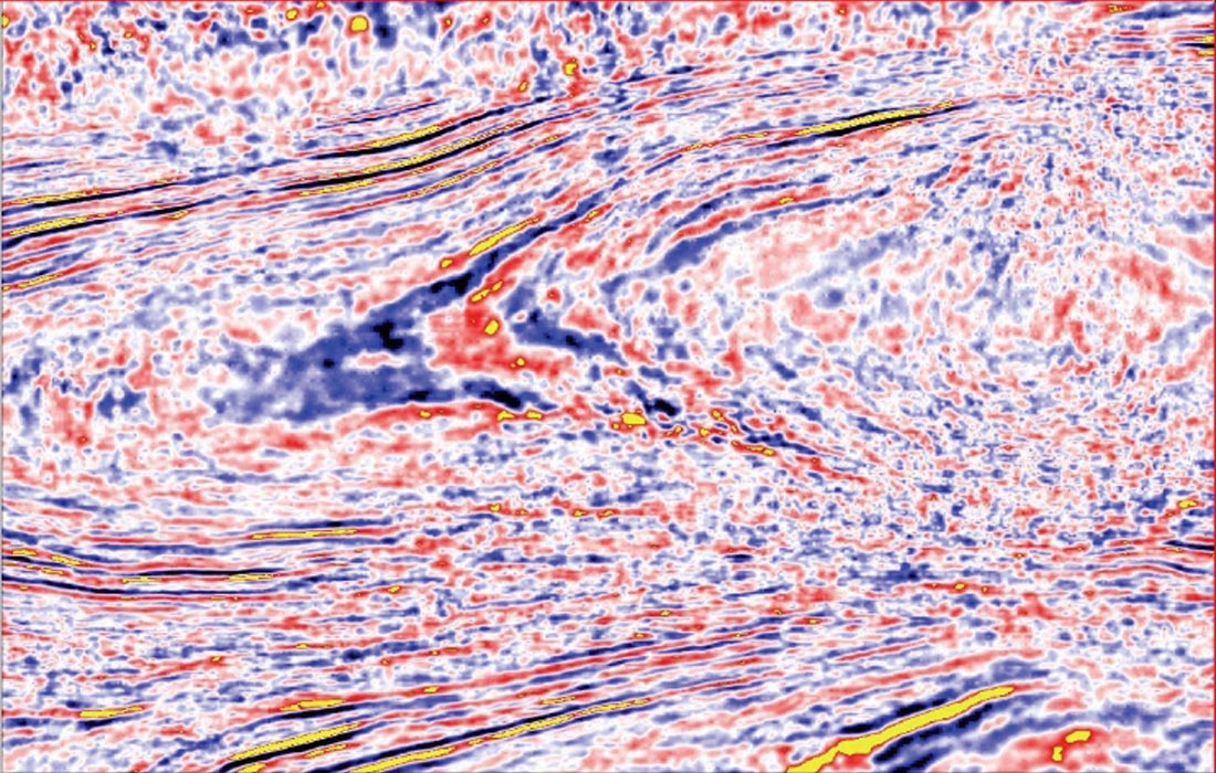
Figure 1 shows an inline of a 3D stack of the complete prestack data being the ‘hidden’ control reference, and a subset of its amplitude spectrum. Spectrum |D| is taken around the area marked by the green circle. Since it is difficult to display the full 5D spectrum, only a 3D subset is shown. The data is 60-fold and has a trace spacing of 25 m. A 1-second window is displayed. Conflicting diffraction curves with different amplitudes are present on both the left and right sides of the figure.

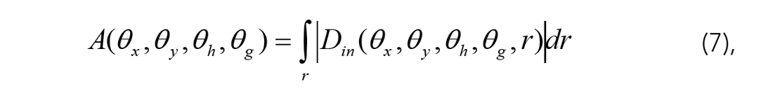
Figure 2 is the stack of input CMP gathers regularly 3:1 decimated in the crossline direction. Consequently, only 33% of the original CMP gathers are used, and are treated as input to the 5D and 6D interpolation tests. The steeply dipping diffraction curves become aliased inside the two yellow highlighted circles. In the middle part of the stack, the gently curved diffractions are not aliased. The incomplete data amplitude spectrum from the right yellow circled area is also shown. The straight yellow dotted arrows in Figure 2’s spectrum will be explained after the Figure 3 discussion.

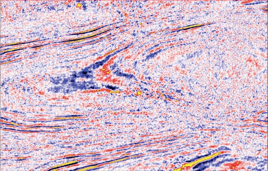
Figure 3 shows the data recovery results of conventional 5D interpolation by MWNI, and the corresponding recovered amplitude spectrum. In order to preserve local structural details, 5D interpolation was done using small time-space data blocks. The results show good recovery of gently dipping data at the middle area of the section, but poor recovery of aliased steeply dipping data at the yellow highlighted areas.

The main idea of the angular weight method is that dip information is derived from the input incomplete data spectrum through calculating the angular sum A. This dip information is imposed back on the input incomplete data spectrum to correct for aliasing by applying the angular weight gamma γ. Referring back to the observed incomplete data spectrum of Figure 2, the straight yellow dotted arrows indicate how one of many angular sums A is found by integrating along that Fourier-radial direction starting from origin using equation (7). It is essentially a dip scan scheme in the five dimensional frequency-wavenumber domain. The dotted arrows in fact can go beyond any Nyquist wavenumbers and wrap around in order to connect the aliased energies of the dipping events.

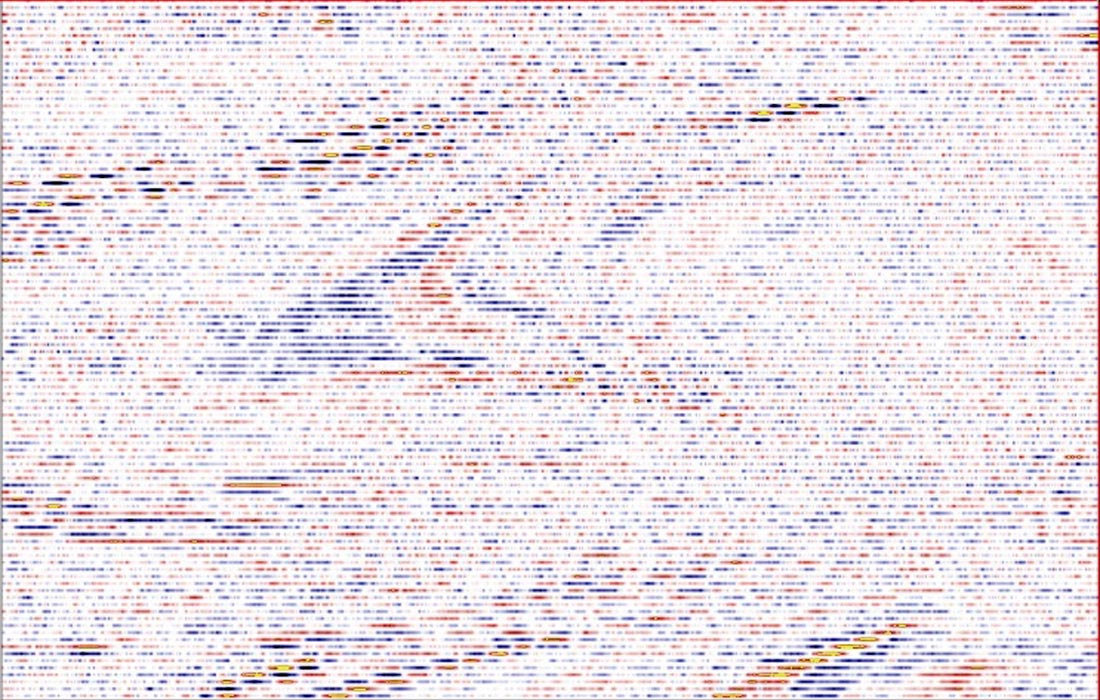
Figure 4 illustrates a subset of the fully measured 5D angular weight gamma γ by populating the 4D angular sum A as described in equation (6). Then, the gamma γ is used to filter the input spectrum in order to give a ‘best’ estimation of the fully sampled data spectrum – the a priori as described in equation (5) for 6D AwMWNI.

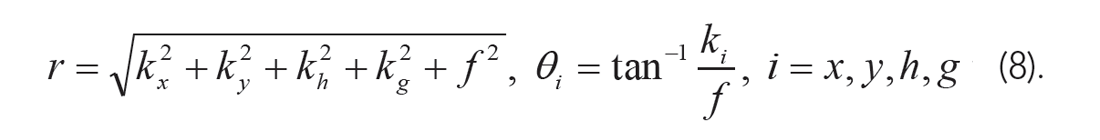
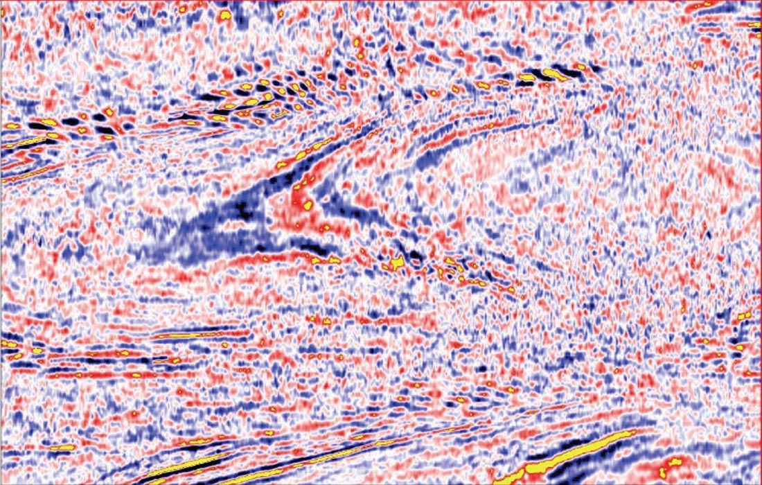
Figure 5 shows the data recovery results by the proposed 6D interpolation by AwMWNI, and the corresponding recovered amplitude spectrum. Identical data blocking parameters are used as for the previous 5D method (Figure 3). In this example, the run time is about 40% more than that of conventional 5D interpolation due to time required for angular weight calculation and application. The proposed 6D interpolation recovery results are very acceptable when compared to the control reference shown in Figure 1.

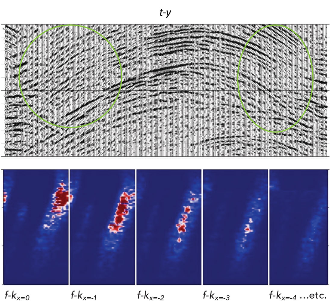
Figure 6 is a composite close-up look at the right circled areas of Figures 1, 2, 3 and 5. This illustrates the performance differences in detail between the 6D interpolation and the conventional 5D interpolation methods for recovering missing structural data in a highly decimated situation.

Figure 7 displays a set of time slices from the top quarter level of Figures 1, 2, 3 and 5, obtained by the above various methods: (a) is a control reference time slice extracted from the original data set corresponding to Figure 1; (b) is a time slice from the 3:1 decimated stack corresponding to Figure 2, and the red circles indicate severe deficiencies in the imaging; (c) is a time slice from the conventional 5D MWNI recovery corresponding to Figure 3; significant data aliasing is found in the top red circle, and poor data recovery is found in the lower red circle; (d) is a time slice obtained from the 6D AwMWNI recovery corresponding to Figure 5; here in the green circles highlighted areas, the data are well de-aliased, and structures are preserved when compared to the reference (a).

Example 2

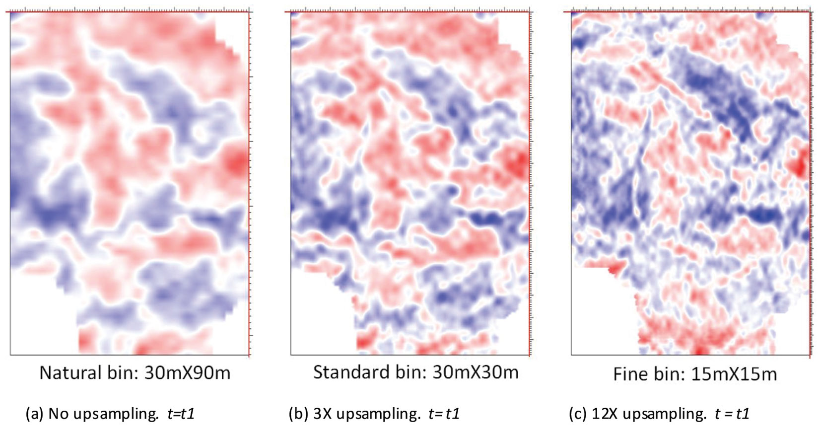
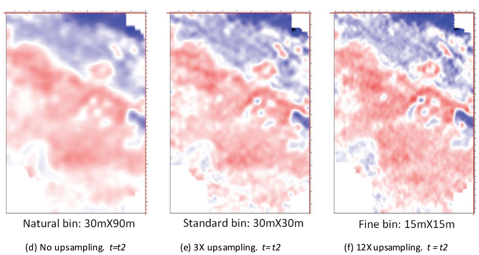
The second example is taken from a production Mega-Bin data set and shows how 6D interpolation can improve spatial resolution by outputting to a finer bin grid than standard Mega-Bin processed bin grid. This was achieved by an ambitiously large upsampling of the input data.

The original Mega-Bin was shot with the 60 m shot and 60 m geophone intervals along the same line running, and a line spacing interval of 180 m. The ‘natural’ bin size is 30 m by 90 m, and the fold is 55. The industry standard Mega-Bin processing will upsample the data 2X conservatively, or 3X in this case, in order to give a regular ‘standard’ bin size. Here, we not only use 6D interpolation to upsample 3X to the 30 m by 30 m ‘standard’ bin size and an output fold of 300, but also use the 6D interpolation to upsample 12X to a 15 m by 15 m ‘fine’ bin size and an output fold of 300.

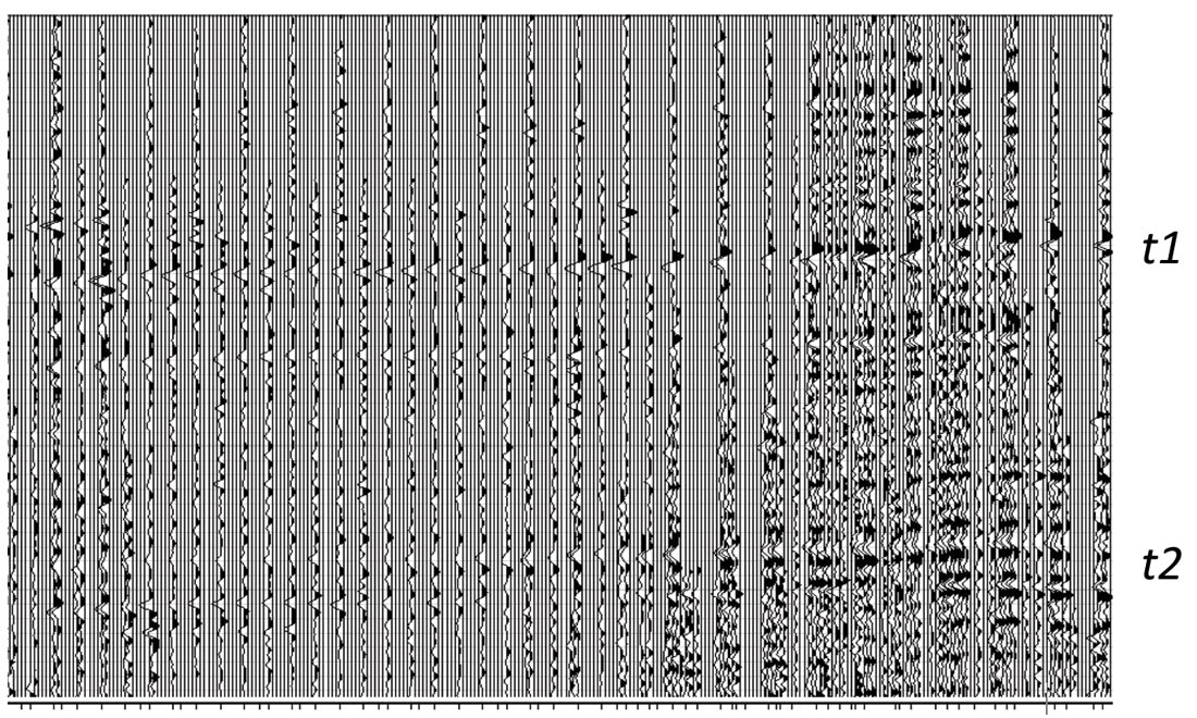
In Figure 8a, an inline of the stack covering 1 second of data is shown, revealing many empty gaps before 6D interpolation of the Mega-Bin data. In Figure 8b, the corresponding inline of the stack after 6D interpolation of the Mega-Bin data upsampled 12X to the 15 m by 15 m ‘fine’ bin size. The data were then post-stack migrated, and the time slices are shown in Figure 9. These time slices shown in Figures 9c and 9f reveal that both resolution and structural clarity improve significantly when a 15 by 15 m ‘fine’ bin grid is output from 6D interpolation when compared to the industry 30 by 30 m ‘standard’ bin grid shown in Figures 9b and 9e. We find that 6D interpolation performs exceedingly well in many situations, surpassing normal upsampling results and achieving finer bin sizes within seismic signal spatial resolution limits, especially for Mega-Bin data.

FAQs

1. Is 6D interpolation AVO compliant?

It is. The Fourier reconstruction MWNI engine, used in 6D AwMWNI, is one of the best, if not perhaps the best, engine for preserving AVO. It can adapt to abrupt amplitude changes within a gather. It provides a resolving power of close to one trace spacing, whose resolution exceeds general AVO variation requirements and structure changes before migration. The manufactured traces at the original input location resemble all characteristics of the original traces extremely well, including the noise. It is like extracting the ‘DNAs’ from the original traces and cloning them onto the interpolated traces. The angular weight Aw part of the dip guide is crucial for stabilizing the non-unique estimation of structures across empty input gathers to be filled in, as well as the empty offset traces to be filled in within a gather.

2. Which one is a better choice: common offset azimuth (COA) grid or common offset vector (COV) grid?

Both polar co-ordinate COA and Cartesian coordinate COV (which is also known as offset vector tile OVT) are favorites in subsurface gridding for multidimensional interpolation. Before interpolation, the fold distributions of both COA and COV are similar; thus they give a similar stack response.

After interpolation, COA gathers have an equal fold distribution across the offset-azimuths, which does not come from a physical geometry. Then, with (or without) Kirchhoff migration, COA grid fits perfectly for its transpose from COCA grid for VVAZ, AVAZ, and HTI analyses, but the stack response is altered when compared to that without interpolation, due to the changed emphasis of actual data in fold distributions which leads to a slightly smooth result.

In the case of COV grid interpolation, the output maintains similar physical fold distributions, loaded with mid-far offsets range which leads to a similar stack response to that before interpolation. Since interpolation with COV grid is closer to a physical geometry, it is more naturally suited than COA grid for interpolated traces to be easily extracted to give additional shots and geophones, on top of the original, for 2D and 3D wave equation shot profile migrations.

Conclusions and looking forward

The 6D interpolation, in contrast to the conventional 5D interpolation by MWNI, has an additional angular weight function dimension that connects dipping data information across all frequency-wavenumbers, which in effect can delineate aliased data in highly structural and deficient-in-data-support situations. This idea can lead to improvements in other frequency-space interpolators as well.

Furthermore, the 6D interpolation leads to an important application: a natural CMP grid size can be subdivided by half in both directions, and 6D interpolation can be used for upsampling to achieve effective resolution of the data without actual field acquisition on the finer grid size. This could result in substantial savings in acquisition costs of up to four times. “It’s comparable to a 1080p high-definition television producing an effective 2160p ultra-high resolution at a small cost.” (Ng and Negut, 2016b).