Stacked tight sands and unconventional plays tend to be found together in what has been termed as deep basin environments also known as continuous basin-centered gas accumulations (BCGAs) which tend to be found predominately in foreland and intracratonic basins but are not restricted to these basins.
There are four geological factors that need to be looked at to determine the success of these stacked tight sands and unconventional plays:
- fluid phase,
- mineralogy,
- pressure regime and
- rock fabric.
Geology and geophysics are key to understanding these geological factors and to locating where these sweet spots exist within the sub-surface. Currently, these sweet spots are drilled into from strategically placed pads. To be able to properly plan both the optimal surface location of the pad and the horizontal well, the time seismic needs to be converted to depth. This can be done using:
- Velocity model built from well data such as sonic logs, check shots, or vertical seismic profiling (VSP);
- Combination of well data and seismic data to be able to better interpolate the velocity data between the wells using geology and geophysical constraints; and
- Prestack depth migration.
The strength of the prestack depth imaging is it handles lateral velocity variations in the overburden between wells. This will position the zone of interest better both horizontally and vertically, which reduces the risk of getting out of zone. When the bit gets out of zone an adjustment needs to be made to get back into zone and this is referred to as “porpoising” because it resembles a porpoise breaking the surface of the water to breathe and then going back into the water. Staying in the zone of interest or the best rock will also increase production (Rauch-Davies, 2018).
One of the products of depth imaging is tomographic velocities that improve the spatial resolution of the seismic velocity field.
There is also automatic high density high resolution continuous (AHDHRC) velocities which can be used on prestack time or depth data, such as Swan velocities. Swan velocities corrects for the velocity error within the AVO gradient and updates the velocities. Swan velocities are residual velocities and may change the velocities by as much 10%. The use of AHDHRC velocities produces flatter gathers that can enhance vertical and horizontal resolution in the seismic, and, if the velocity field is overlain on the seismic data, can bring out the nature of the fault, be it a sealing fault or leaky fault, and illuminate zones that may be overpressured.
Introduction
The drop in the price of oil, from $95/bbl in 2014 to $45/bbl in 2017, caused exploration and production (E&P) companies to search for ways to lower their costs per barrel oil equivalent (BOE). The E&P companies needed to produce the oil more economically to significantly reduce their break-even-points (BEP) for conventional and unconventional plays.
Lower BEPs were driven both by technological advances in how companies drilled and completed wells as described in Table 1, and economic performance. With the lower price of oil, E&P companies were not drilling as much. This created an oversupply of rigs, which in turn caused rig and completion costs to decrease.
| 2010 | 2016 |
|---|---|
| Table 1. Comparison of drilling and completion techniques from 2010 to 2016 taken from Blackbird Energy (2016). | |
| Average number of stages 10 | Average number of stages 25 |
| Average length of lateral 1250 m | Average length of lateral 2000 m |
| Average spacing of stages 125 m | Average spacing of stages 75 m |
| Fluid pumped 2500 m3 | Fluid pumped 15000 m3 |
| Proppant placed 750 tonnes | Proppant placed 15,000 tonnes |
| 20% of the wells use slick water | >70% of the wells use slick water |
| Completions used perf and plug which tends to be more time consuming due to trips to prepare each zone hydraulically fracked. | Completions used open hole ball drop systems which allow the well to be completed in a single continuous process; less water is required. |
| Energizing of the fracturing fluid with N2 or CO2 which reduces the amount of water necessary to induce fracking and improves flowback since the invaded water saturation is lower. | |
From 2013 to 2016, the drop in BEP was partly due to the following technological advances to drilling and completion wells:
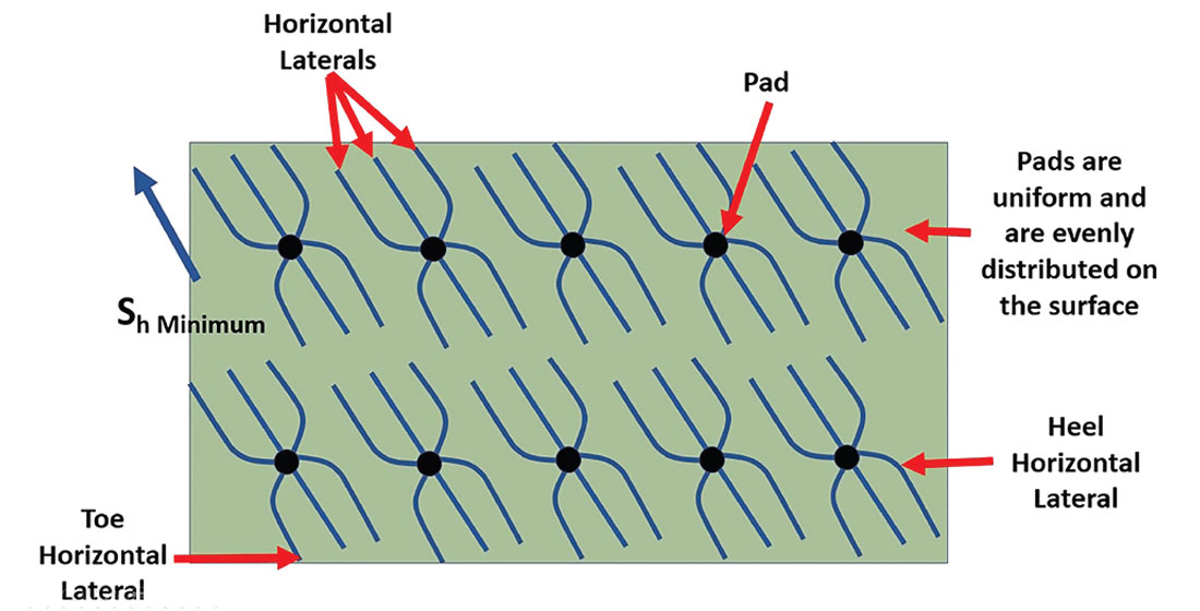
- Pad drilling, that utilize one location to drill multiple horizontal wells.
- Longer horizontal wells being drilled twice as fast, compared to 5 years ago.
- Changes in the configuration of the horizontal wells, i.e. length, number of stages, amount of fluid used, amount of proppant placed. For example, in the Eagle Ford, the more sand pumped, the greater the production profile (Mason, 2018).
- Changes in completions techniques, such as zipper fracks, where fracturing operations are carried out concurrently on two horizontal wellbores that are close and parallel to each other.
- Choke management during flowback, that restrict flow rates in the short term, but produces a flatter production profile and larger cumulative production in the long term, producing a better type curve.
Unconventional plays are often drilled using a cluster of horizontal wells drilled from strategically placed pads as displayed in Figure 1, to maximize the recovery from the acreage with minimal disruption to the surface conditions.
Unconventional Plays and Geology
There are several definitions of unconventional plays, but this paper considers an unconventional play to be a special category which implies the use, or potential use, of advanced drilling and/or completions technology to make it economic (Seifert, 2012).
Successfully exploiting an unconventional reservoir depends upon:
- Storage capacity of the rock, which is dependent upon the porosity, which is generally linked to the generation of hydrocarbons which creates pore space within the kerogen grains (Williams, 2012; Romero-Sarmiento et al., 2013), and expulsion, which creates microfracture networks (Williams, 2012).
- Permeability, which can be pressure dependent (Vera Rosales, 2012).
- Potential for fracture stimulation. The conduits for fluid to flow within tight unconventional plays to the induced fractures are the porosity and the natural fractures (Lohr et al., 2015).
Frack-ability or Potential for Fracture Stimulation
There are three geological factors that need to be looked at to increase the “frack-ability” of an unconventional play:
- Mineralogy: Brittle minerals like silica (e.g. quartz), dolomite, and to a lesser extent calcite, break like glass, while clay minerals are more ductile, absorb more of the pressure, and often bend under applied hydraulic pressure without breaking.
- Pressure Regime: If the formation is overpressured, the artificially created fracture network can penetrate further into the formation because the formation is more critically stressed than a normally pressured formation.
- Rock fabric: This includes the natural fractures, bedding, geomechanical properties (Poisson Ratio, Young’s Modulus, brittleness, etc.), stress orientation, etc. that can be estimated using elastic properties, azimuthal and geometric seismic attributes.
Foreland Basins / Deep Basin Geology
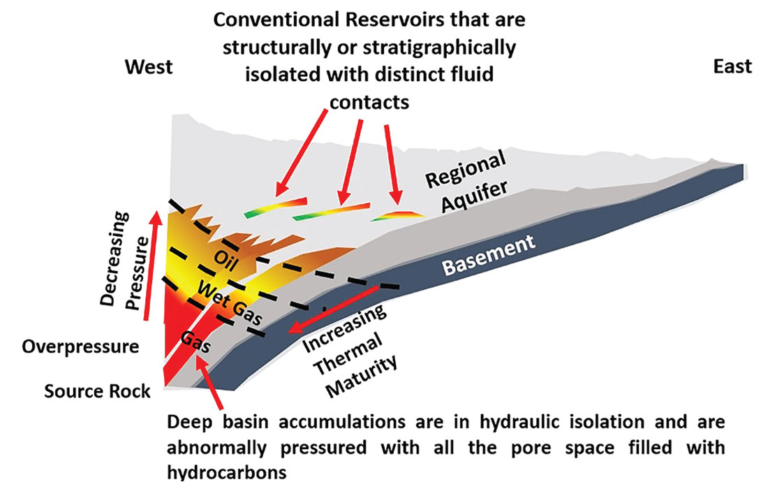
A foreland basin is a structural basin that develops adjacent and parallel to a mountain belt. It is formed due to lithospheric flexure, which is caused by the immense mass created by crustal thickening during an orogeny. The foreland basin receives sediment eroded off the adjacent mountain belt and the craton, filling the basin with thick sedimentary successions that thin away from the mountain belt and the craton (Figure 2).
It is believed that, due to the rapid subsidence of rocks, foreland basins are cooler than normal, with relatively lower geothermal gradients and heat flow. This is important in the maturation and generation of hydrocarbons. Examples of foreland basins with prolific hydrocarbon accumulations include the following:
- Anadarko Basin, underlying the western part of Oklahoma and the Texas Panhandle, extending into SW Kansas and SE Colorado.
- Appalachian Basin, containing the Marcellus Shale.
- Deep Basin in Western Canada, containing the Montney.
As mentioned, deep basin environments also known as continuous basin-centered gas accumulations (BCGAs) (Law, 2002; Schmoker, 2005; Zee Ma, et. al., 2016) tend to be found predominantly in foreland and intracratonic basins but are not restricted to these basins.
The Deep Basin in Western Canada is home to:
1. Stacked, tight, clastic reservoirs:
These were deposited in a foreland basin during the Mesozoic (e.g. Cardium, Dunvegan, Viking, Cadotte, Notikewin, Falher, Bluesky, Gething, Cadomin, Nikanassin, Rock Creek and, in NE BC, the Halfway) and are channel or shoreface sands. The source rocks are the surrounding shales and coals. The shales tend to contain Type II kerogen that is formed from marine organic materials and spores and pollen of land plants. It produces both oil and gas. The coals tend to contain Type III kerogen that is formed from terrestrial plant material, lacks lipids or waxy material, and produces gas. Type III kerogen generates a higher GOR than the oil-prone kerogens, but the oil-prone kerogens (Type I and II) can generate twice as much hydrocarbon gas per gram of organic carbon as the Type III kerogen (Lewan and Henry, 1999).
2. Unconventional plays:
- Wilrich: The Cretaceous Wilrich was deposited in the foreland basin and has Type III kerogen. It tends to be shoreface sandstones that are fine- to medium-grained, well-sorted, feldspathic litharenite to lithic arkose. Up to 30% of the bulk fabric of the rock is plagioclase, with the plagioclase being the brittle mineral. The Wilrich tends to be difficult to see on seismic data due to the overlying coal which produces strong sidelobes that interfere with the seismic signature of the Wilrich Formation.
- Doig: The Triassic Doig Shale is up to 11% TOC, particularly in the radioactive phosphate zone (Walsh, et al., 2006; Ibrahimbas and Riediger, 2004; Faraj et al., 2002) and has Type II kerogen. Sometimes production from the Doig Phosphate is combined with the underlying Upper Montney siltstones and sands.
- Montney: The Triassic Montney may have been deposited in a passive margin, back-arc or fore-arc setting (Rohais, et. al., 2016) and has Type II kerogen.
- Duvernay: The Paleozoic Duvernay was deposited in a passive margin setting and contains Type I and II kerogen. Type I kerogen provides the highest yield of oil and forms from: alginite; amorphous organic matter; cyanobacteria; freshwater algae; and land plant resins.
The formations in the Western Canada Deep Basin, and most other deep basins / BCGAs, are in hydraulic isolation and are abnormally pressured with all the porosity filled with hydrocarbons at sub-irreducible water saturation. The hydrocarbon-bearing sands grade laterally updip into permeable water-bearing sands without any reservoir barriers to segregate the fluids, so gas is under water (Gies, 1984). This change is the major difference between deep basin / BCGAs and conventional accumulations of hydrocarbons. Conventional reservoirs are isolated structurally and stratigraphically with distinct fluid contacts (Hillis, et al., 2001).
Overpressured Zones
In deep basins / BCGAs, during the maturation of the source rock, the pressure will build, and the formations will become overpressured (Burnie, et. al., 2008; Zee Ma, et. al., 2016). Once a certain pressure threshold is reached, the gas will begin leaking and escape up dip, reducing the pressure to a normal and ultimately underpressured state (Burnie, et. al., 2008; Zee Ma, et. al., 2016) when the amount of gas being produced is lesser than the amount that is escaping.
Overpressure tends to be the most important component in deep basin environments or continuous basin-centered gas accumulations (BCGAs) because it increases the porosity (Edwards et al., 2015) and the permeability of the formation. It also allows the artificially created fracture network to penetrate further into the formation.
Being able to identify zones that are overpressured within the formation using seismic data will affect potential production.
Effect of Pore Pressure on Production
During production, the pore pressure is decreased, and this produces complicated relationships with permeability; generally, as pore pressure decreases it reduces the permeability due to rock compaction. If the pore pressure is drawn down too fast, proppant embedment may occur, which reduces the performance of the horizontal well; implementing aggressive choke management will improve overall well performance and reserve recovery, improving the type curve (Cherry, 2018).
This can help explain the term “frac hit”, which is interference between lateral wells that causes a decline in production in the older lateral well. Part of this decline may be due to the rapid bleeding off of the pore pressure in the older lateral well, rapidly closing the permeability, causing proppant embedment and closing some of the induced fractures.
Unconventional Plays in Alberta / British Columbia
This paper will focus on the Montney and the Duvernay, although the Wilrich is also an important resource play in Alberta, and the Doig Phosphate zone is being considered as an upcoming new resource play.
1. Montney. The Montney is geologically younger than the Duvernay. The Montney resource play is in the Deep Basin and is both over- and under-pressured. It is brittle and stiff due to the silica (45-60 % quartz) and dolomite content so it fractures easily. The Montney has different fluid phases (Figure 3).
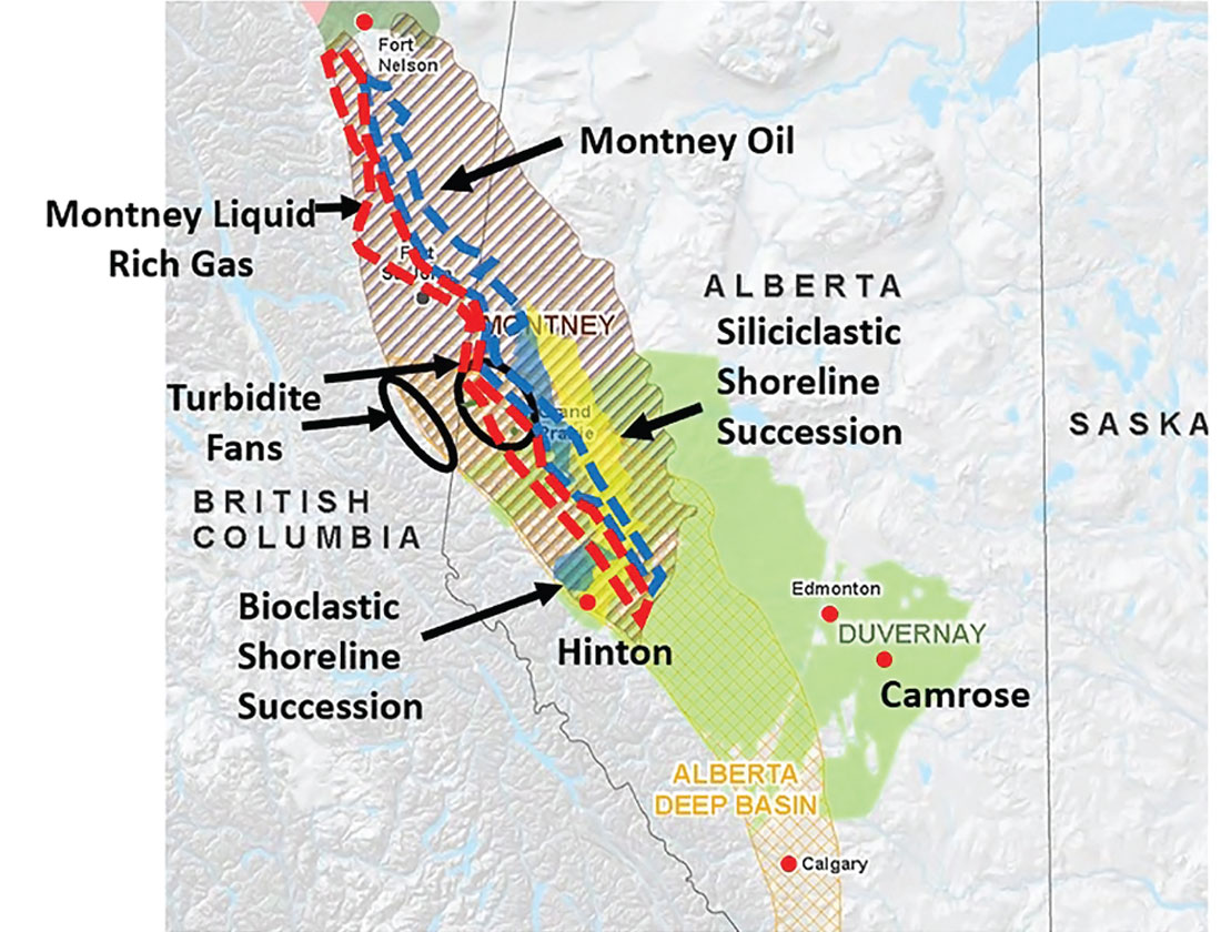
The Montney is self-sourced with the hydrocarbons not migrating very far, due to very low permeabilities (Euzen et al., 2015). Porosity in the Montney may have been created in part by thermal maturation (intra-kerogen porosity). Good porosity within the Montney yields a higher drilling rate of penetration (ROP) which infers the ability to drill horizontal wells faster. It is 300 m thick with multiple pay zones (minimally upper, middle and lower).
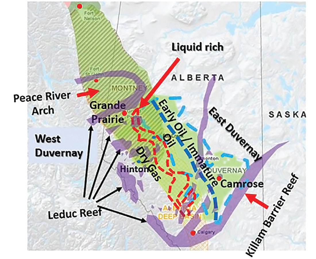
2. Duvernay. Like the Montney, the Duvernay has different fluid phases (Figure 4) and it can be broken into two plays, the West Shale Basin Duvernay and the East Shale Basin Duvernay:
- West Shale Basin Duvernay
The West Shale Basin Duvernay (WSBD) is predominately a sequence of gray mudrocks with one dominant carbonate interbed; it is in the over-pressured Deep Basin with pressures up to 80% above hydrostatic (Rokosh et al., 2012; Watson, 2017) and no significant water in the system; it is deeper, and it produces a liquid rich gas (Rokosh et al., 2012; Watson, 2017). What makes the WSBD as attractive as the Texas Eagle Ford play is that the Duvernay can produce significant volumes of liquids due to its overpressured nature (Dunn et al., 2013). The Duvernay was deposited in areas proximal to reef development (Dunn, et al.,2013). The reefs created restricted basin conditions where organic activity was high creating thick, high TOC deposits that were deposited in anoxic conditions (Dunn et al., 2013), preserving the organic matter. - East Shale Basin Duvernay
The East Shale Basin Duvernay (ESBD) is thinner, thermally less mature because it is shallower, and is in a region with a lower geothermal gradient. The shale tends to be in the oil window, have higher carbonate content which lowers the geothermal gradient, and has inconsistent pressure/depth ratios with moderate over-pressuring to slightly under-pressured tests and water cuts (Watson, 2017).
The successful wells in the East Shale Basin Duvernay tend to be in the light oil window. The problem with black oil in shales is due to shale’s micropermeability, the black oil’s viscosity, and the lack of reservoir energy. These factors make it hard to sustain commercial flow rates in black oil shale plays (Dembicki, 2014). In black oil shale plays, the production tends to come from highly fractured sand or carbonate stringers. These stringers tend to be easily fracked compared to the shales.
Use of Seismic
The goal of seismic usage is to use basic interpretation techniques to identify sweet spots within tight sands and unconventional plays and plan the horizontal well path as efficiently as possible so it will intersect the best rock and avoid potential pitfalls during fracking.
AVO and Partial Stacks
The Deep Basin is a gas-filled basin, and rocks filled with gas tend to have an AVO signature. The AVO anomalies present in the Deep Basin tend to be Rutherford and Williams (1989) Class 2, Class 2P and Class 1 AVO (Figure 5), due to the hardness of the rock.
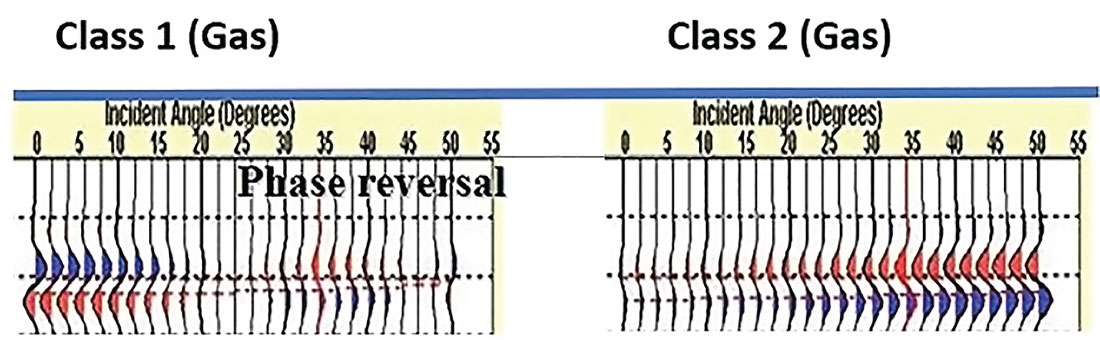
Most geophysicists use the full stack because it tends to have the highest signal to noise ratio which is the result of higher fold or number of traces being summed together to create each stacked trace in the stack. Unfortunately, there are issues with just using the full stack because summing all the offsets together will destroy any indications of amplitude variations with offset (AVO), especially Rutherford and Williams (1989) Class 1, Class 2 and Class 2P as shown in Figure 5.
Partial stacks are an effective proxy for a full (and expensive) AVO analysis of gathers.
Geohazards and Faults
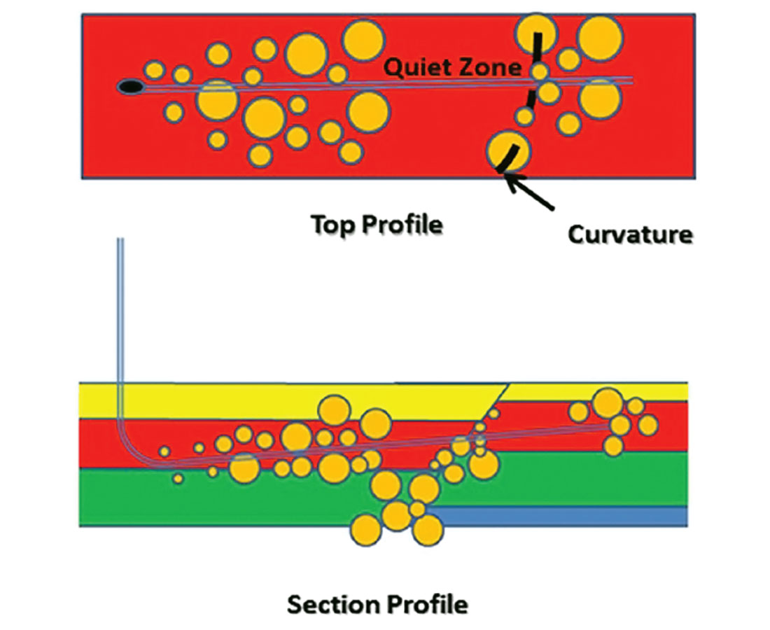
Seismic can also be used to identify geohazards for the horizontal well, such as salt dissolution, karsting and faults. Faults can be beneficial or can act as thieves, allowing the frack fluids and proppant to escape down the fault plane, as shown in Figure 6, and in some instances, cause induced seismicity.
Conversion of Time to Depth
The planning of the horizontal well is done in depth. Most seismic data are processed as time data, so it needs to be converted to represent depth to be used for horizontal well planning.
Most geophysicists utilize sonic well logs, check shots and VSPs to create an interval velocity field which can convert (“stretch”) time seismic data to depth. The main weaknesses with this are:
- Lateral velocity variations in the overburden between wells (Rauch-Davies, 2018) creates false push-downs or pull-ups in the imaging of the zone of interest. This could lead to the drill bit being out of zone during drilling.
- The interpolation of the well log velocities from one well to the next is not based on any geological or geophysical information.
Issues with Dix Equation (1955)
Dix equation (1955) is traditionally used to convert the VRMS or stacking velocities to interval velocities. The issue with the Dix Equation (1955) is it produces laterally unstable, geologically unrealistic and oscillating interval velocities (Koren and Ravve, 2005; Schulte, 2012). Several approaches have been developed for the inverse Dix transform to prevent anomalous values of interval velocities from easily corrupting the entire inversion and they are referred to as Constrained Velocity Inversion (CVI). These approaches generally follow Harlan’s (1999) algorithm using least squares which produces a smooth interval velocity field (Koren and Ravve, 2005; Schulte, 2012).
Using Well Logs and Seismic Velocities in Unison
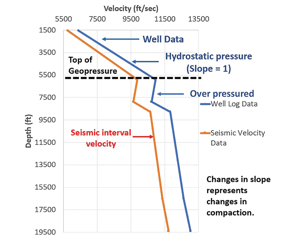
The seismic interval velocities created using CVI should be delivered in ASCII and SEGY format (interpolated to match the 3D seismic cube and sampled at the same sample rate as the seismic) to the interpreter at the end of the processing, so it can be compared to the sonic log interval velocities. The values should not match in value but the general trend / slope of the velocities should.
When there are changes in the pressure in the subsurface, there is a change in the linear trend or slope of the interval velocities and some refer to this as changes in the compaction trend. When the compaction trend follows hydrostatic pressure (slope of 1), it is said to be normally pressured. When it deviates from hydrostatic pressure it is either over or under pressured.
The reason why the values between the sonic log interval velocity and the seismic interval velocity are not the same is because sonic log data are vertical velocities and seismic velocities are horizontal velocities. The difference between the two is due to the anisotropy of the rock and is generally within 10% (Figure 7).
A calibration factor can be calculated by comparing the seismic velocity at the well location to the sonic log. The seismic interval velocity is typically 10% less than the velocity from the sonic log. The calibration factor can be applied to the seismic velocities. This converts the seismic velocities to vertical rock velocities. This creates a better velocity field that can be loaded into the interpretation software. In some interpretation software, the seismic velocities can be co-kriged with the sonic log interval velocities to produce a velocity field that is based on geology and geophysics. This velocity field, based on seismic interval velocities and calibrated to the sonic well log, provides a better interpolated velocity field which considers both geology and geophysics and allows for better interpolation away from the sparse well control.
This co-kriged velocity field can be used for converting the time data to depth and it will better represent the geology than a velocity field created using only well data.
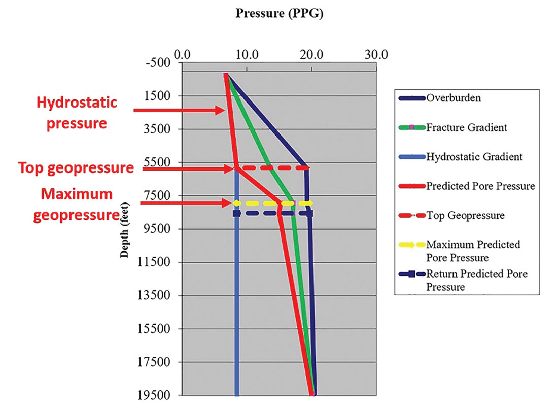
Geopressure
As the pore pressure in the rock increases, it approaches the fracture gradient (Figure 8) which makes the rock easier to break. The fractures may be easily induced, penetrating deeper into the rock formation which will result in better production.
Prestack Depth Migration
According to Rauch-Davies (2018) the strength of prestack depth imaging is that it handles lateral velocity variations between wells. This allows the zone of interest to be better positioned in the seismic and reduces the risk of getting out of zone. Staying in the zone of interest will also increase the production. Prestack depth imaging is also used to achieve better resolution of subtle faults.
Depth Imaging By-Products
Two by-products that come from depth imaging are:
- Anisotropic model, that represents the sub-surface geology (Rauch-Davies, 2018)
- Velocity model, built using reflection tomography which utilizes a general ray-trace model-based approach (Bishop et al., 1985; Stork, 1992; Wang et al., 1995; Sayers et al., 2002; Chopra and Huffman, 2006; Schulte, 2018) that improves the spatial resolution of the seismic velocity field (Sayers et al., 2002; Schulte, 2018). This can be used to understand overpressures across the 3D and help plan the vertical section of the well to determine the mud weights for drilling.
Automatic High Density, High Resolution, Continuous (AHDHRC) Residual Velocities
Some operators are also using automatic high density, high resolution, continuous (AHDHRC) residual velocities on prestack time or depth migrated data calculated such as Swan’s (2001) residual velocity indicator (RVI), that reduces the error within the gradient due to residual velocity (Spratt, 1987; Swan, 2001; Schulte 2018).
Since Swan (2001) velocities do not rely on semblances or on improving the moveout but on reducing of the velocity error in gradient, it tends to be able to calculate better velocities for the Class 1, 2P and 2 Rutherford and Williams (1989) AVO anomalies which tend to be predominant in the Deep Basin.
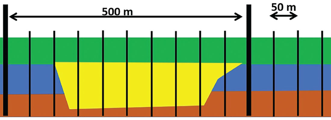
Picked velocities are generally done on a spatially coarse sampled grid, which causes the loss of the short wavelength variation in the stacking velocity field (Suaudeau, et al., 2002) which is illustrated in Figure 9. This may lead to poor stacking in areas where there are strong lateral variations in the seismic velocities and the blurring of subtle faults.
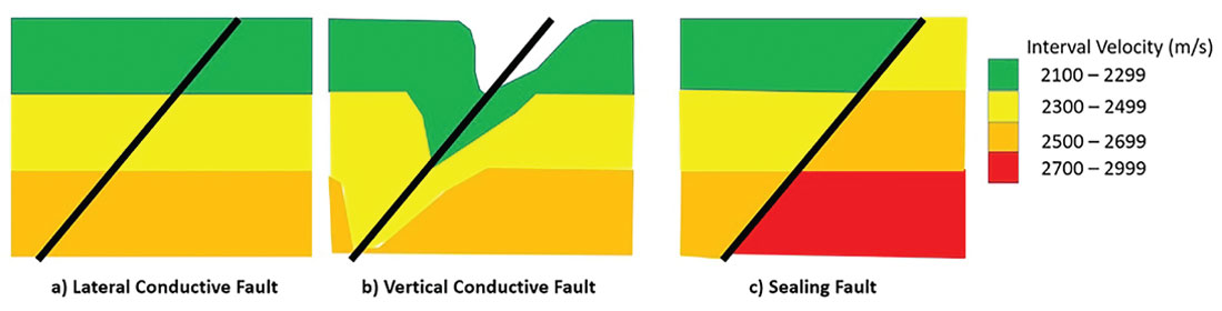
The AHDHRC velocity field can aid in the interpretation. Overlaying the high-density continuous interval velocities (such as those generated by a CVI) onto the seismic will bring out subtle features such as the presence of overpressures distributed laterally, or the nature of a fault: laterally conductive fault (leaky fault), vertical conductive fault, or a sealing fault (Figure 10) (Kan and Swan, 2001; Schulte, 2018).
Conclusions
Overpressure is an important factor, because when the formation is near formation fracture pressure, artificially induced fracture networks may penetrate further into the formation. Therefore, using seismic to identify zones of overpressure should enhance the accuracy of production prediction. Using calibrated tomographic or AHDHRC seismic interval velocities, it is possible to identify location and extent of overpressured zones, determine the nature of a fault's pressure communication, and illuminate possible compartments. This method has been proven in the Gulf of Mexico through the work of Kan and Swan (2001).
Use of partial stacks allows for the use of AVO analysis and the identification of possible sweet spots within the shales. Being able to identify sweet spots allows for better planning of the horizontal wells.
To be able to plan the horizontal well properly the seismic data needs to be in depth. This can be done using:
- Velocity model built from well data such as sonic logs; check shots; and VSP’s;
- Utilization of well data and seismic data to be able to better interpolate the velocity data between the wells using geological and geophysical constraints; and
- Prestack depth migration.
The overlaying of CVI interval velocities, be them tomographic or AHRHDC, onto the stacks will help identify overpressured zones. Sometimes where there is overpressure there will be a noticeable AVO anomaly in the data. This AVO is due to an increase in porosity and permeability, due to the overpressure pushing the sediment grains apart within the formation. Porosity creates a conduit for fluids to flow within tight unconventional plays to the induced fractures (Lohr et al., 2015).
Overpressure is an important component because the formation is near naturally fracking, and any artificially induced fracture networks will penetrate further into the formation. Thus, being able to use seismic to infer zones that are overpressured should positively affect potential production. This can be done using calibrated tomographic or AHDHRC seismic interval velocities to infer overpressured zones and possibly determine its lateral distribution; help identify how fault behave; and, illuminate possible compartments. This method has been proven in the Gulf of Mexico through the work of Kan and Swan (2001).

Acknowledgements
I wish to thank Neil Watson at Enlighten Geoscience; George Fairs at Divestco Inc.; Ruth Peach, Technical Editor for CSEG RECORDER; and Albert Scutt for helping with the edits of this paper and challenging myself on how the material was presented.


Join the Conversation
Interested in starting, or contributing to a conversation about an article or issue of the RECORDER? Join our CSEG LinkedIn Group.
Share This Article